Visualization of 2D data
2D Image Visualization Workshop: Fiji & Napari
Table of Contents
- What is Fiji?
- Getting Started with Fiji
- Opening and Viewing Images
- Essential Fiji Functions
- Alternative: Napari in Jupyter Notebooks
What is Fiji?
Fiji (Fiji Is Just ImageJ) is a free, open-source image processing and analysis platform built on top of ImageJ. It’s widely used in scientific research, particularly in microscopy, medical imaging, and general image analysis.
Key Features
- User-friendly GUI - No programming required for basic operations
- Pre-installed plugins - Comes with a curated selection of image processing tools
- Extensible - Can add additional plugins for specialized tasks
- Multi-format support - Handles TIFF, JPEG, PNG, BMP, and many scientific formats
- Batch processing - Automate workflows with macros
- Active community - Extensive documentation and forum support
Common Use Cases
- Microscopy image analysis
- Segmentation and thresholding
- Intensity measurements and statistics
- Image registration and stitching
- 3D image visualization
- Time-series analysis
Getting Started with Fiji
Download and Installation
Windows, Mac, or Linux
- Visit the official Fiji website: https://fiji.sc/
- Click “Download” and select your operating system
- Extract the downloaded file to your preferred location (preferably somewhere admin rights are not required to modify files)
- Double-click
Fiji.exe(Windows) or the Fiji application bundle to launch
No additional installation required - Fiji is portable and comes with Java bundled.
Verify Installation
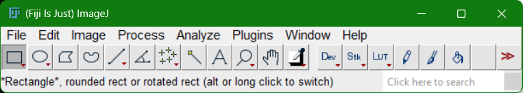
When you launch Fiji, you should see: - The main ImageJ window (toolbar with various tools) - A menu bar with File, Edit, Image, Process, Analyze, Plugins, Window, Help
Setting Up Sample Data
For this workshop, we recommend having sample images available. You can: - Use your own microscopy images or photographs - Use Fiji sample data - Download sample images from: - Fiji sample images - Scientific image repositories (e.g., Open Microscopy Environment)
Opening and Viewing Images
Opening an Image
The easiest way is to use drag-and-drop on the gray area.
Another option is to:
- File → Open (or
Ctrl+O/Cmd+O) - Navigate to your image file and select it
- Click Open
The image will display in a new window with the filename in the title bar.
In many cases, the BioFormats Plugin will be automatically called to open the image.
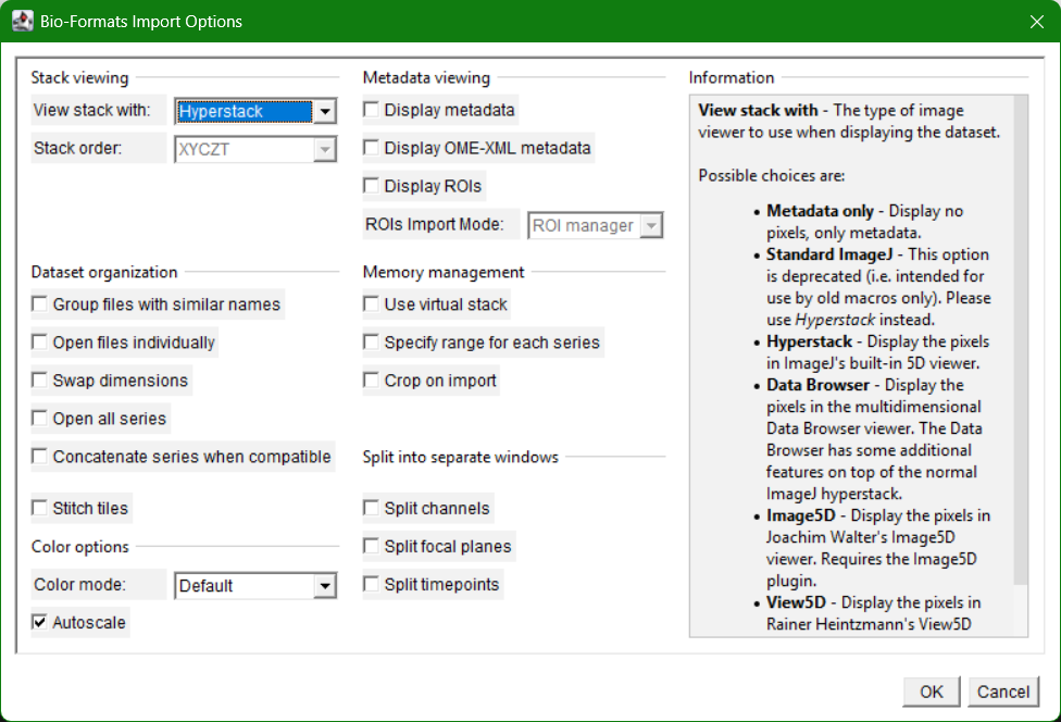
How many of these options do we understand?
Basic Viewing Tools
| Tool | Function | Shortcut |
|---|---|---|
| Zoom In/Out | Adjust magnification to inspect details or see whole image | + / - or scroll wheel |
| Pan | Move around the image when zoomed in | Click and drag with spacebar |
| Color Picker | Sample pixel values | I key |
| Measure | Determine distances and areas | M key |
| ROI (Region of Interest) | Select rectangular, oval, or free-form areas | Toolbar buttons |
Excercise
Zoom in as much as you can into a small region. What do you see? Are the squares part of the sample or a rendering? If you hover your mouse over some pixels, what do you see at the bottom grey area of the Fiji main window?
Checking Image Properties
After opening an image, first check its header. What are the values on top?
Can you check its metadata? (go to Image>Show Info...)
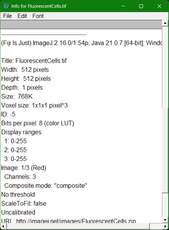
Fill in the following table:
| Metadata Item | Value |
|---|---|
| Pixel Size (µm) | |
| Magnification | |
| Numerical Aperture (NA) | |
| Bit Depth | |
| Image Dimensions (width × height) | |
| Number of Channels | |
| Number of Slices (if z-stack) | |
| Voxel Dimensions | |
| Unit |
Changing the Bit Depth
Images can be stored in different formats representing different levels of intensity information:
- 8-bit (256 intensity levels) - Smallest file size, fastest processing, good for display
- 16-bit (65,536 intensity levels) - More detail, larger file size, common in microscopy
- 32-bit (floating-point) - Highest precision, largest file size, used for calculations
To change the bit depth of your image:
- Go to
Image > Type - Select your desired bit depth:
8-bit,16-bit, or32-bit - If converting from higher to lower bit depth (e.g., 16-bit to 8-bit), you may lose information
Exercise
Why might you want to convert a 16-bit image to 8-bit? Consider factors like file size, processing speed, memory usage, and the type of analysis you plan to do. When would it be a bad idea?
Essential Fiji Functions
Duplicate an image
Most of the operations are applied on the currently selected image, which might change its intensity values. Some operations cannot be undone, which means that you have to reopen the image and go through the whole process again if something goes wrong. To avoid this, it’s a good idea to duplicate the image just in case.
Go to Image > Duplicate.
Adjusting Brightness & Contrast
Image > Adjust > Brightness/Contrast...- Drag sliders to enhance visibility
- Check Auto for automatic adjustment
- Use Reset to revert to original
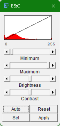
Use case: Make dim images more visible for analysis.
Excercise
Try clicking on Apply to see what happens to the pixel values.
Changing the LookUp Table
Most of the cameras or detectors are monochromatic, which means that the color with which images are represented is a false color. Go to Image > LookUp Tables or click on the LUT button and choose a different color. What do you think the different palettes are for? Try for example HiLo, cool and 16-colors.
Working with more dimensions
First choose an image with several dimension, like a z-stack with more than one channel. If you don’t have one, you can choose File > Open samples > Mitosis (5D stack).
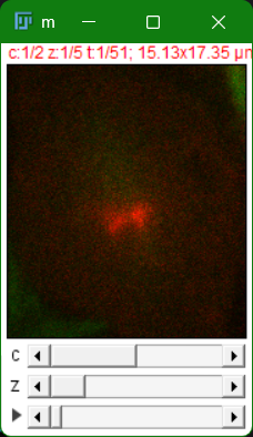
The sliders at the bottom allow you to go through the different channels, z-planes and timepoints. Some of the sample images already have what is called a composite, where channels are shown simultaneously. Try doing the following:
Split Channels
Image > Color > Split Channels- Each channel opens in a separate window
- Analyze or process channels independently
Merge Channels
Image > Color > Merge Channels- Select source windows for each channel
- Do not create a composite image
Channel Visualization
- Adjust color assignments for better visualization
- Go to
Image > Color > Make Composite
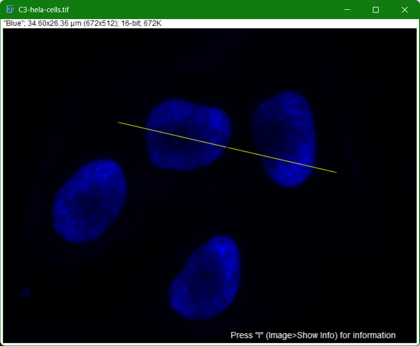
Quick Measurements
Choose any structure in your image.
- Click on straight line button
- Draw a line across your object of interest
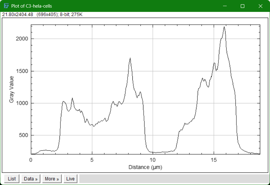
- Go to
Analyze > Plot Profile - Displays intensity values along the line (useful for colocalization studies)
What happens if you right click on the straight line button?
Measure Intensity
- Select an ROI (Region of Interest) using selection tools
- Analyze → Measure (or
Ctrl+M) - Results include: Area, Mean intensity, Std Dev, Min, Max
Crop
- Use rectangle selection tool to define region
- Image → Crop
- Image is reduced to selected area
Alternative: Napari in Jupyter Notebooks
If you prefer a Python-based, interactive approach, napari is a fast, interactive image viewer for multi-dimensional images.
Installation
Pixi is a package manager that makes it easy to manage Python environments and dependencies. Follow these steps to set up Napari with pixi:
Install Pixi
Visit the official Pixi website: https://pixi.sh/
Download and install Pixi for your operating system (Windows, Mac, or Linux)
Verify installation by running in your terminal:
pixi --version
Initialize a Pixi Project
Create a new directory for your image analysis project:
mkdir my-image-analysis
cd my-image-analysis
Initialize a Pixi project:
pixi initThis creates a
pixi.tomlconfiguration file for your project.
Add Python and Napari to Your Environment
Add Python, napari, and Jupyter to your project:
pixi add python napari jupyter scikit-imageThis command: - Installs Python and the specified packages - Creates a pixi.lock file with exact versions for reproducibility - Sets up an isolated environment specific to your project
Running Jupyter with Pixi
Start Jupyter notebook directly from your pixi project:
pixi run jupyter notebookThis runs Jupyter within your project’s environment, giving it access to napari, scikit-image, and all other packages you added.
Basic Napari Workflow
Import and Display an Image
import napari
from skimage import io

# Load an image
image = io.imread('path/to/image.tif')

# Create viewer and add image layer
viewer = napari.view_image(image, name='raw image')
Interactive ROI Selection
We can do this either programatically from within the Jupyter notebook, or we can do this interactively from the Napari GUI.
import napari
from skimage import io

image = io.imread('path/to/image.tif')

viewer = napari.Viewer()
layer = viewer.add_image(image)

# Add shapes layer for ROI drawing
shapes_layer = viewer.add_shapes(
    shape_type='rectangle',
    edge_color='cyan',
    face_color='transparent',
    name='ROIs'
)
Or:
- Click on the button to generate a new Shapes Layer
- Add a new rectangle
Once the rectangle is made, try accessing it via a cell in the Jupyter notebook. Access drawn shapes via shapes_layer.data.
Napari Advantages
- Interactive - Real-time parameter adjustment
- Jupyter integration - Works in notebooks for reproducible workflows
- Python-native - Easy integration with scientific Python stack (scikit-image, scipy, etc.)
- Multi-dimensional - Handles time series, z-stacks, and multi-channel data
- Programmatic ROI - Extract measurements from selected regions in code
Napari Limitations vs. Fiji
- Less pre-built analysis functions (requires coding)
- Smaller ecosystem of plugins compared to Fiji
- Learning curve for Python programming
Additional Workshop Exercises
Exercise 1: Basic Image Inspection (Fiji)
- Download a sample image
- Open in Fiji
- Check image properties (dimensions, bit depth, channels)
- Use zoom and pan tools to explore
- Measure a feature using the measure tool
Exercise 2: Image Enhancement (Fiji)
- Open a dim or low-contrast image
- Apply Brightness/Contrast adjustment
- Apply Gaussian blur to reduce noise
- Use Unsharp Mask to enhance edges
- Compare original and processed versions
Exercise 3: Segmentation (Fiji or Napari)
- Open a 2D image with distinct objects
- Apply threshold to create binary image
- Use morphological operations (Erode/Dilate) to clean up
- Run Analyze Particles to count and measure objects
- Generate summary statistics
Exercise 4: Reproducible Analysis (Napari in Jupyter)
- Load an image using scikit-image
- Apply preprocessing (blur, threshold)
- Perform segmentation
- Visualize results with multiple layers in napari
- Extract measurements from labeled regions
Tips & Tricks
Fiji Performance
- For very large images, reduce memory usage via Edit → Options → Memory & Threads
- Disable auto-update of image window to speed up processing: Edit → Options
- Use 8-bit images instead of 16-bit when precision isn’t critical
Reproducibility
- Document your workflow by recording macro actions: Plugins → Macros → Record
- Export processing steps as macro code for batch processing
Jupyter Best Practices
- Save images and results to standardized output directories
- Use consistent naming conventions for variables
- Document parameters used for each processing step
- Version your analysis notebooks in git
Resources
- Official Fiji Documentation: https://fiji.sc/
- ImageJ User Guide: https://imagej.net/
- Napari Documentation: https://napari.org/
- Scientific Image Analysis Tutorials: https://imagej.net/Tutorials
- Scikit-image (Python): https://scikit-image.org/
Citation
Corbat, A. A. (2026). Workshop on 2D Image Visualization: Fiji and Napari. Zenodo. https://doi.org/10.5281/zenodo.18199646
License
This work is licensed under the Creative Commons Attribution 4.0 International License (CC BY 4.0).
For more details, visit: https://creativecommons.org/licenses/by/4.0/ and https://github.com/acorbat/2D_visualization_workshop
Last Updated: January 2, 2026