Post-processing, segmentation and labelling

Author

Marina Cuenca

Published

January 5, 2026

2D segmentation in Fiji

In this exercise we will:

Compare global and local thresholding methods and understand when each is useful.
Improve segmentation using background subtraction and Gaussian smoothing.
Refine masks using binary operations, including Fill Holes and Kill Borders.
Generate labeled objects using MorphoLibJ’s Connected Components Labeling.
Extract object-level measurements (area, perimeter, circularity, etc.).
Visualize measurement values on labeled images.
Filter segmented objects based on size or other properties.

These steps form a complete workflow: raw image → pre-processing → segmentation → cleanup → labeling → measurement → filtering

We’ll use MAX_Lund.tif as the example image https://zenodo.org/records/17986091

Requirements: - Fiji - MorphoLibJ plugin https://imagej.net/plugins/morpholibj

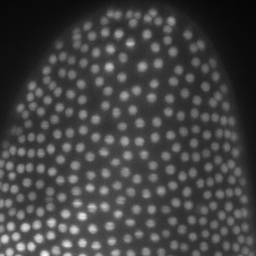
1. Open the image and inspect the histogram

Start Fiji.
Open the image:
File → Open… → MAX_Lund.tif
Open the histogram and visualization tools:
Image → Adjust → Brightness/Contrast…

You should see a histogram like this:

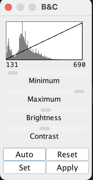
Idea: Thresholding chooses an intensity value that separates “foreground” from “background”. The histogram shows how many pixels exist at each intensity.

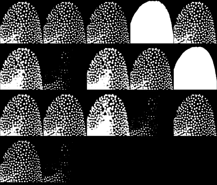
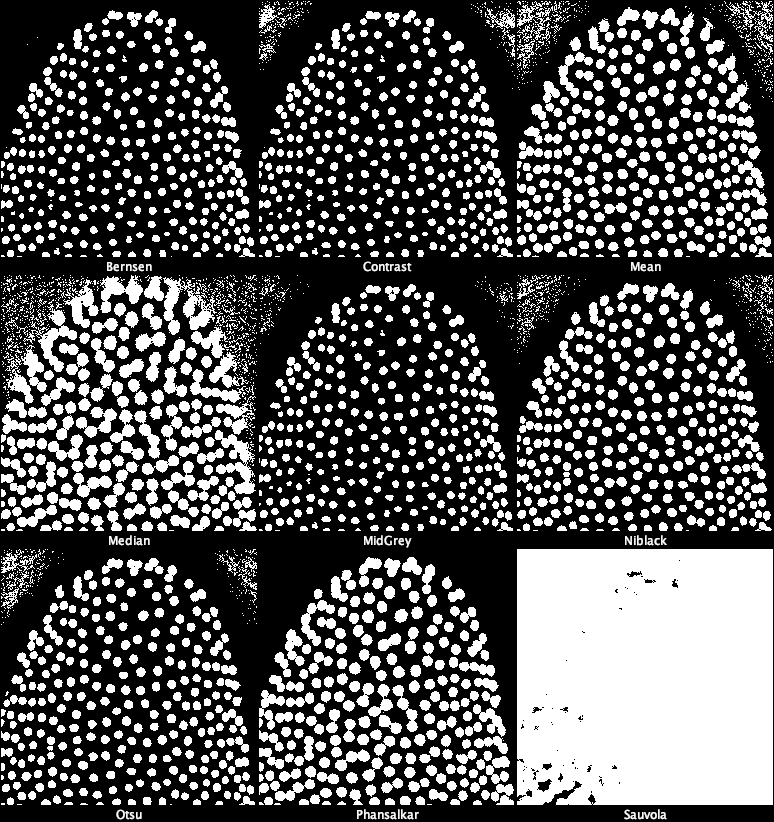
2. Try all global Auto Threshold methods

Global thresholding applies one single threshold to the whole image.

With MAX_Lund.tif active, run:
Image → Adjust → Auto Threshold…
Choose:
- Method: Try all
- White objects
Confirm.

Fiji generates a montage of all global methods:

3. Prepare the image for Auto Local Threshold

Local thresholding requires 8-bit input.

Select the original image:
Window → MAX_Lund.tif
Convert to 8-bit:
Image → Type → 8-bit

Now the image is ready for local methods.

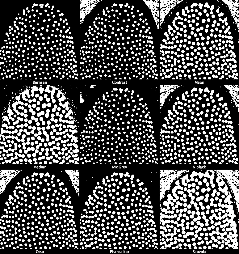
4. Try all Auto Local Threshold methods

Local thresholding computes a threshold for each local neighborhood.

Run:
Image → Adjust → Auto Local Threshold…
Choose:
- Method: Try all
- Radius: 15
- Parameter 1: 0
- Parameter 2: 0
- White objects
Confirm.

5. Improving segmentation with background subtraction and smoothing

Good segmentation often benefits from reducing background and noise first.

5.1 Remove background and apply Gaussian blur

Open MAX_Lund.png.
Subtract background:
Process → Subtract Background…
- Rolling ball radius: 50
Smooth noise:
Process → Filters → Gaussian Blur…
- Sigma: 1

After preprocessing:

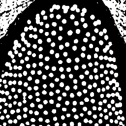
6. Selecting a method: Local Otsu and binary cleanup

6.1 Apply Local Otsu thresholding

Run:
Image → Adjust → Auto Local Threshold…
- Method: Otsu
- Radius: 15

Local Otsu mask:

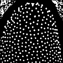
6.2 Refine the mask with binary operations

Fill holes inside objects:
Process → Binary → Fill Holes
Slightly shrink objects:
Process → Binary → Erode
Optionally restore outlines:
Edit → Draw
Expand objects after erosion:
Process → Binary → Dilate

Refined mask:

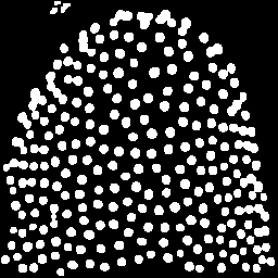
6.3 Remove border-touching objects

Remove partial objects touching image borders:
Plugins → MorphoLibJ → Filtering → Kill Borders

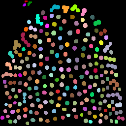
7. Object labeling with MorphoLibJ

Convert each connected region into a uniquely labeled object:

Plugins → MorphoLibJ → Label → Connected Components Labeling

Connectivity: 4
Output type: 16-bit

Labeled objects:

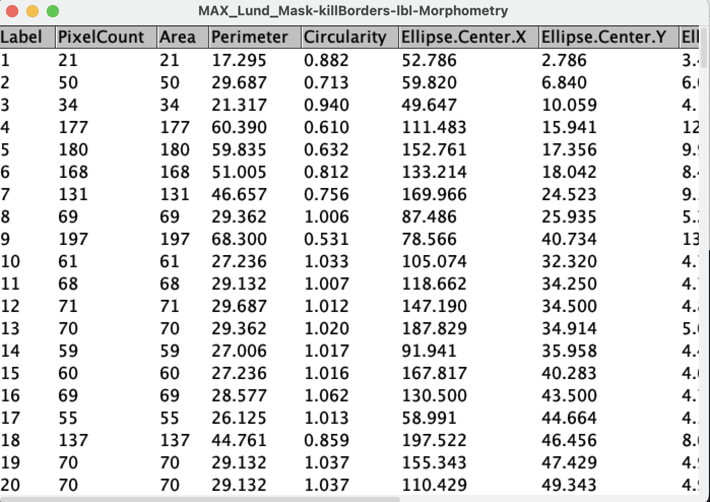
8. Measuring object properties

Quantifying each object is often the main goal after segmentation.

Run measurements:

Plugins → MorphoLibJ → Analyze → Analyze Regions

This extracts a number of morphological associated features. We will select:

Area
Pixel count
Perimeter
Circularity
Ellipse geometry
Bounding box

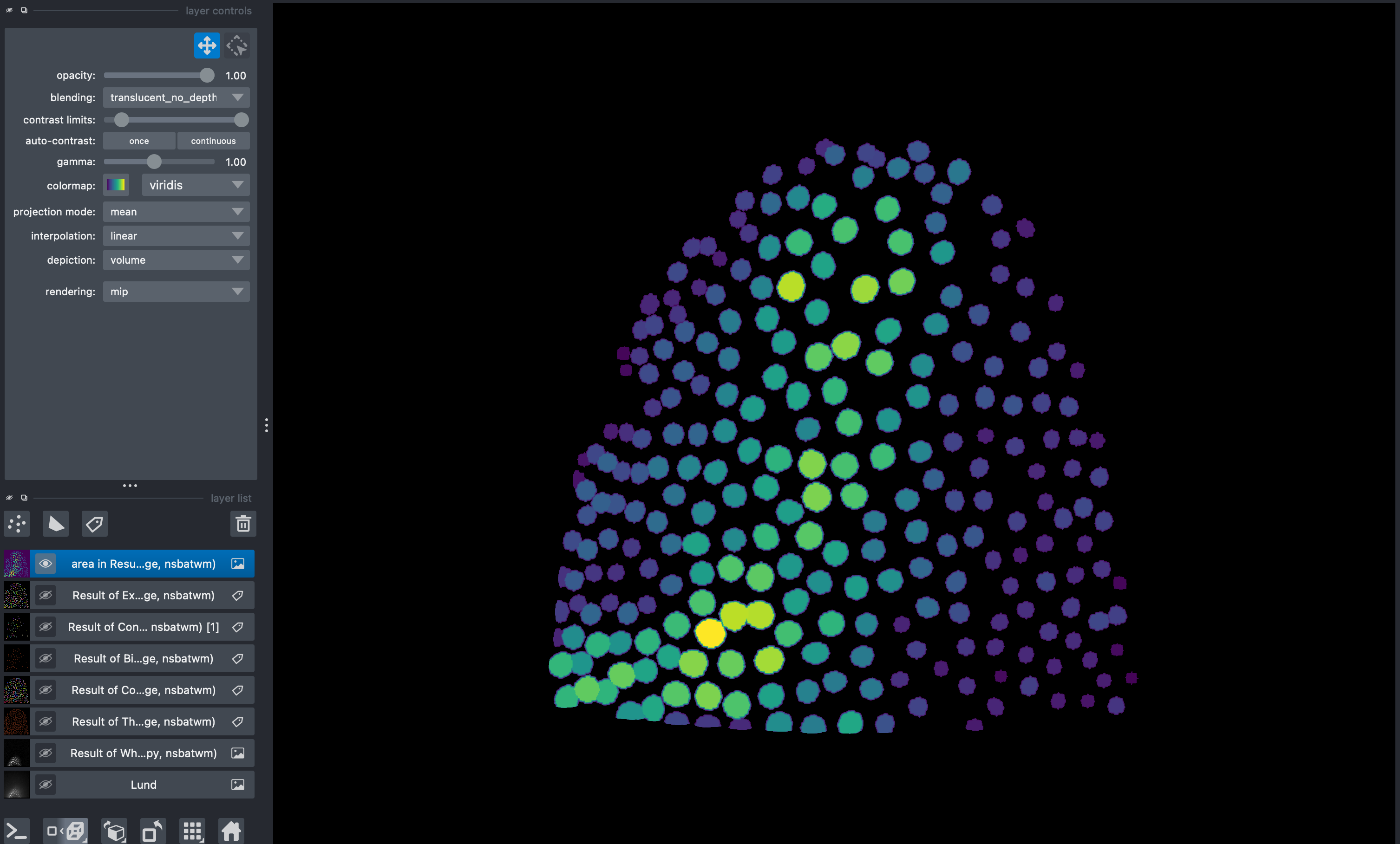
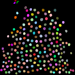
9. Visualizing label properties

Visualize one measurement (e.g. area) mapped onto the label image:

Plugins → MorphoLibJ → Label Images → Assign Measure to Label

Choose Area and apply a colormap.

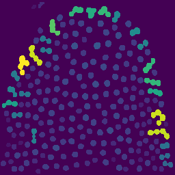
Useful for:

spotting unusually big/small objects
deciding filtering thresholds
checking measurement correctness

10. Filtering objects by size

Remove small objects based on size:

Plugins → MorphoLibJ → Label Images → Label Size Filtering

Operation: Lower Than
Size threshold: 100 px

3D segmentation in Napari

In this exercise we will:

Use Napari to open a 3D image
Use Napari assistant to visualize a workflow for 3D image segmentation and labelling
Use region props to quantify morphological parameters and make colorcoded plots

These steps form a complete workflow:
raw image → pre-processing → segmentation → cleanup → labeling → measurement → filtering

We’ll use Lund.tif as the example image https://zenodo.org/records/17986091.

Requirements: - Everything you need is in the toml file in the Pixi/napari-assistant folder https://github.com/cuenca-mb/pixi-napari-assistant

0. Open Napari assistant using Pixi

In the terminal, go to the directory Pixi/napari-assistant and run:

pixi run assistant

1. Open a 3D stack

Drag and drop the file or

File → Open File

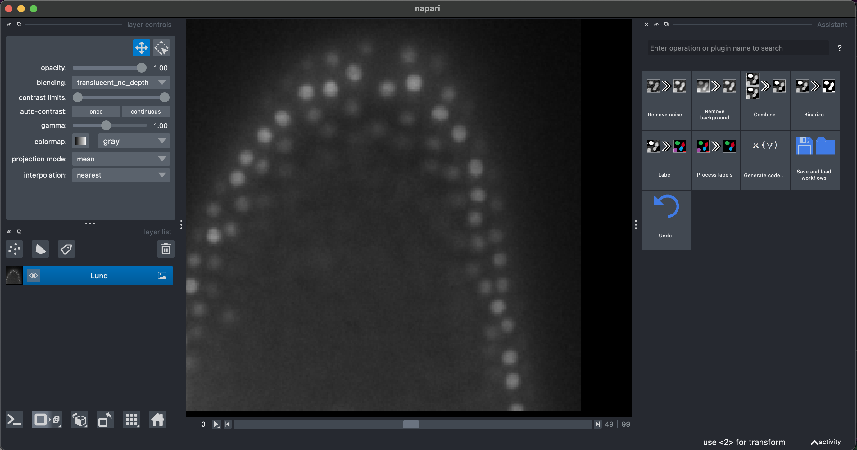
We will be able to see and explore the stack, and we can change to a 3D rendering with the option Toogle 2D/3D view in the lower left button pannel. We can also make orthogonal views by clicking the button to the right Change order of the visible axis.

In the right pannel we will see the Assistant plugin, where it suggests operations in the appropriate order. The amount of operations and options depends on your installed plugins. Some of them are redundant.

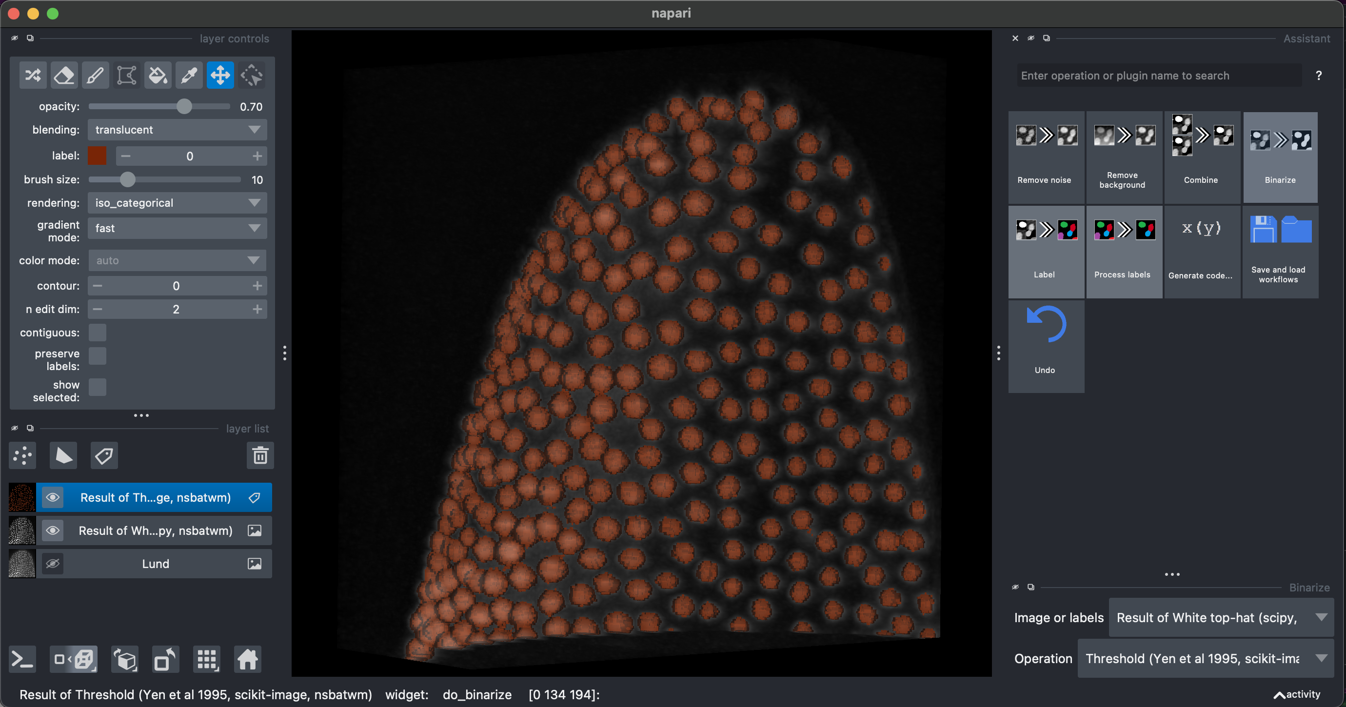
2. Remove background, binarization and labeling

Select Remove Background → White top hat → radius = 10

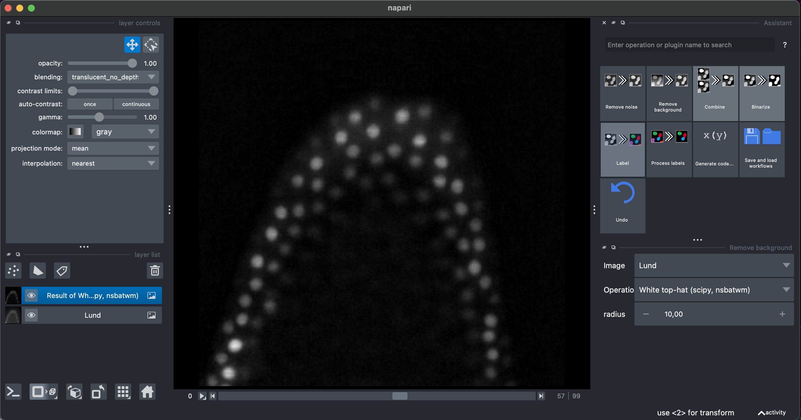
Then select Binarize → Threshold Yen, making sure to select the Result of White top-hat image.

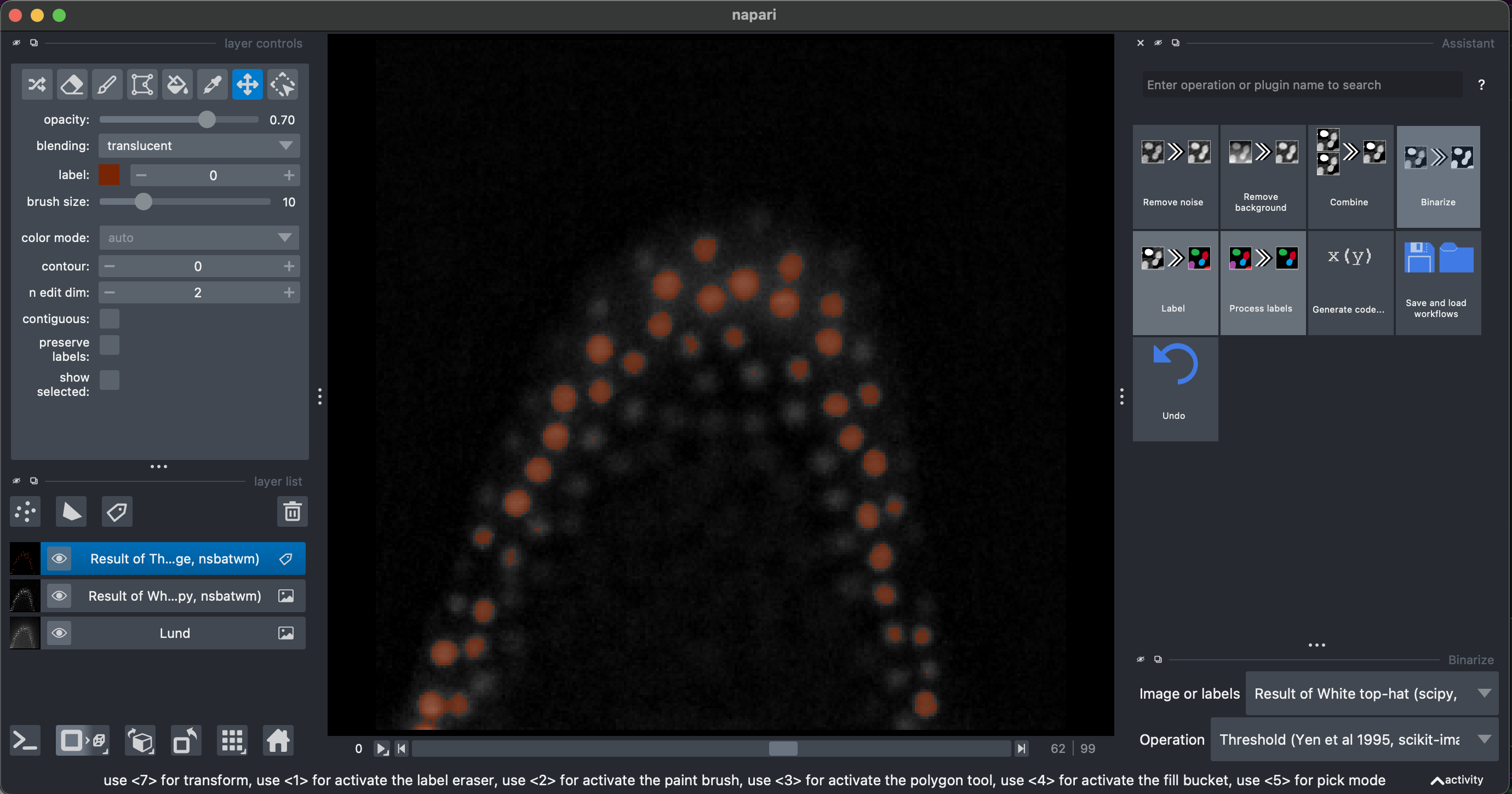
I recommend looking at the result in 3D.

Finally, we can select Label → Connected component labeling, make sure to select the Result of Threshold image. We can additionally select the exclude on edges option.

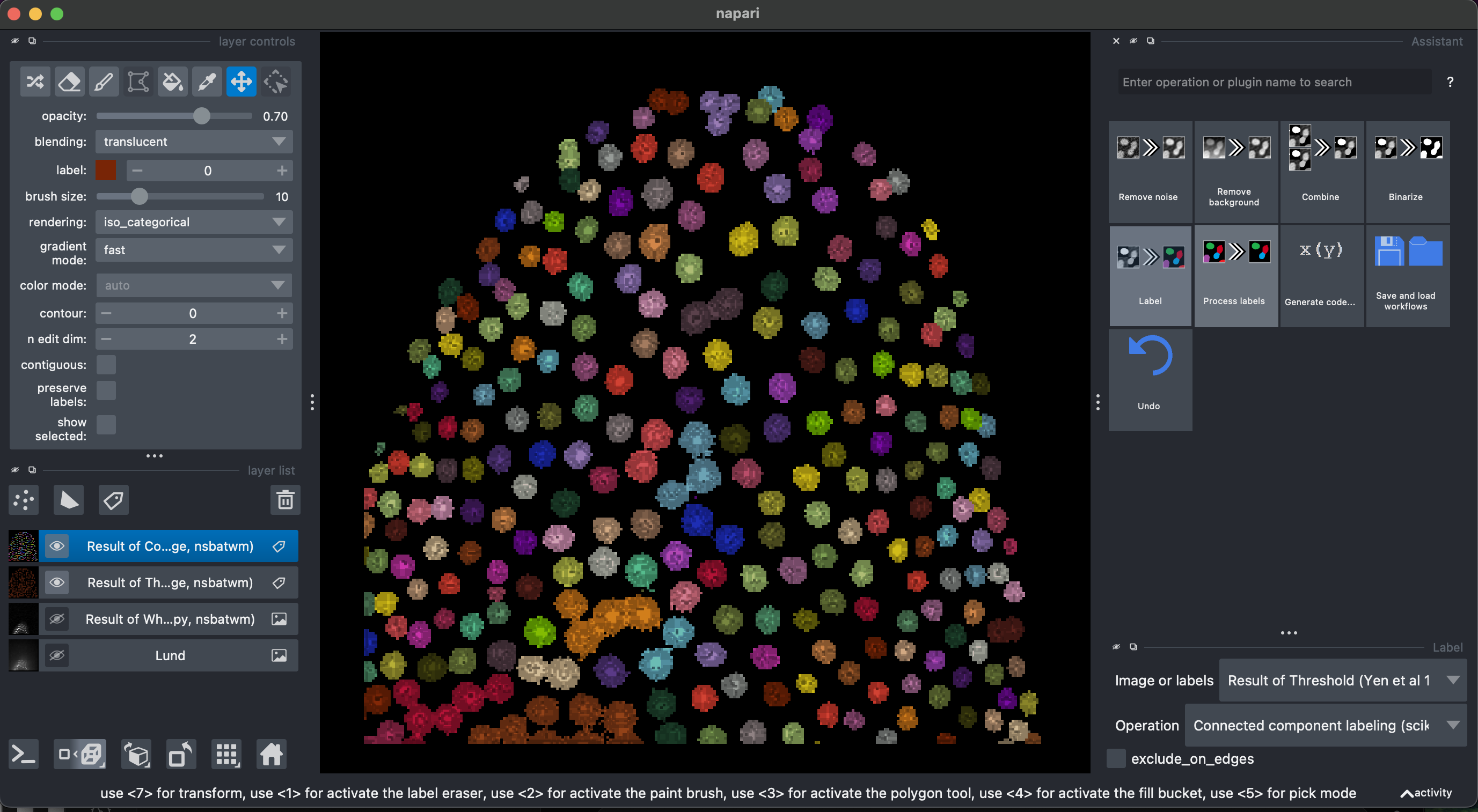
Some of them are stuck together. Let’s try and fix that.

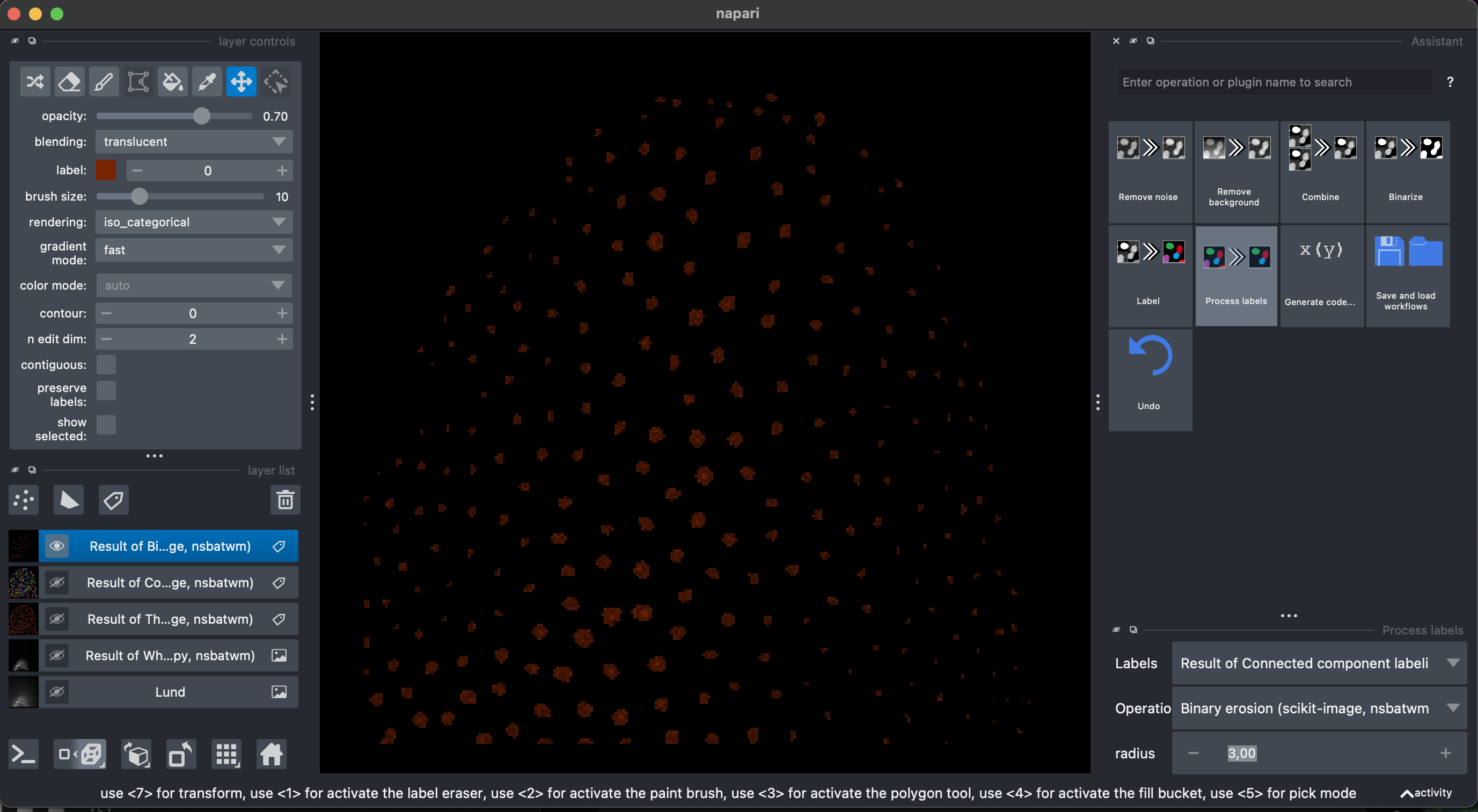
3. Fix labels

Let’s select again the previous layer Result of Threshold. Then select Process labels → Binary erosion → radius = 3. This will reduce the objects of the binary segmentation.

Now let’s recreate the labels Label → Connected component labeling, make sure to select the Result of Binary Erosion.

Then Process labels → Expand Labels → radius = 3. Explore the labels in 3D.

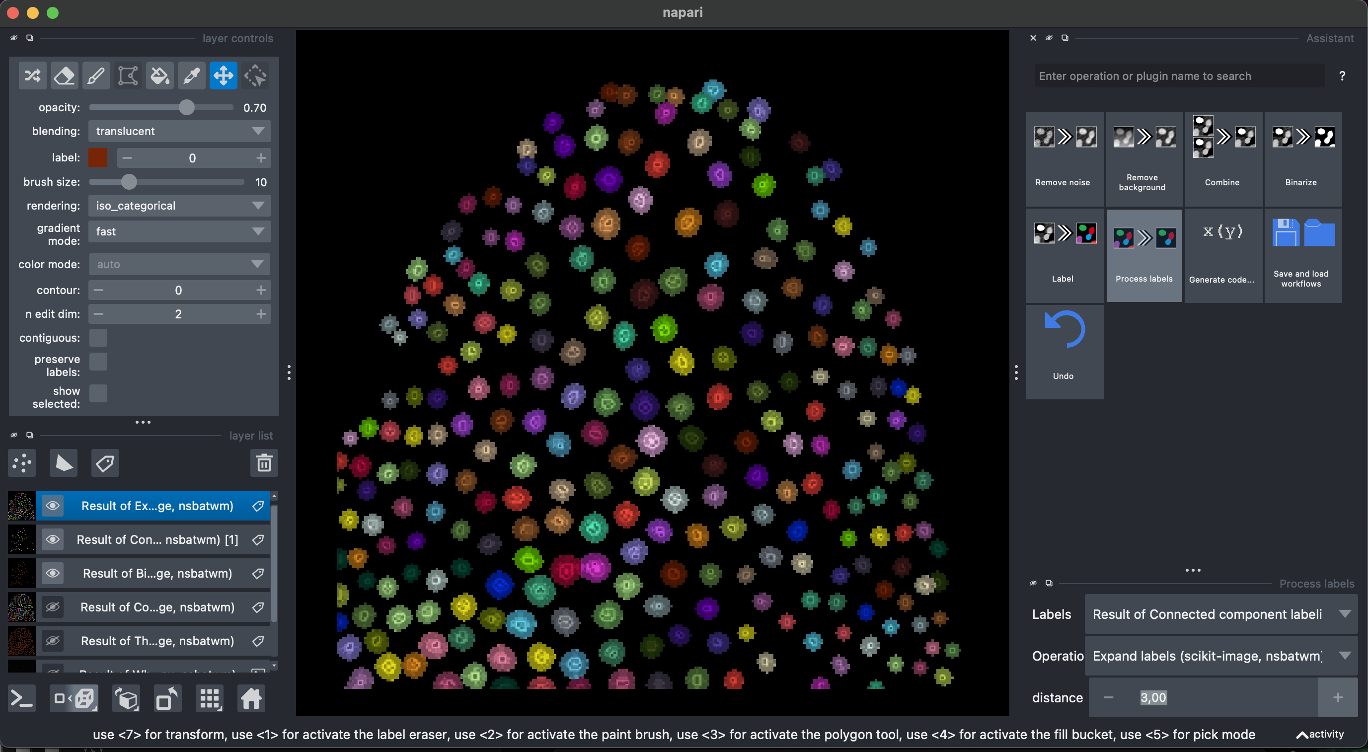
Now we can accurately measure morphological features of these labels. You can close the assistant pannel now.

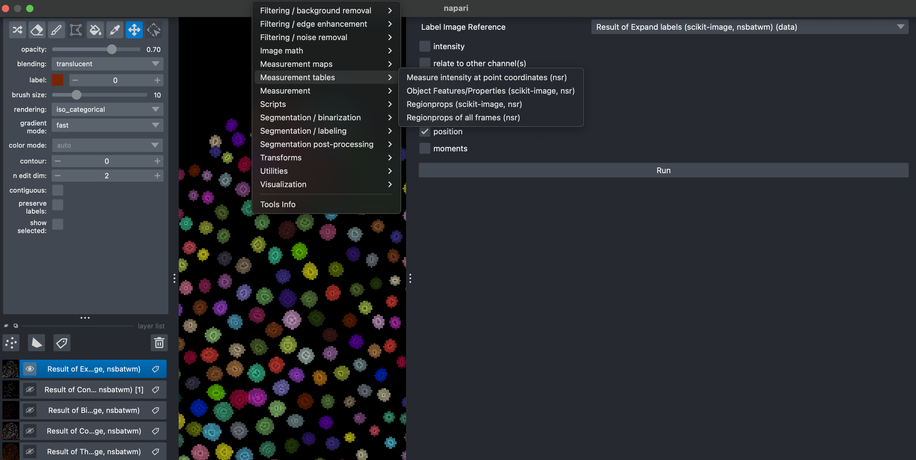
4. Measure morphological properties

Select Tools → Measure Tables → Object Features/Properties. Here make sure to select the Result of Expanded Labels image. You can select different features, includding intensity features extracted from the raw data. After running a table should appear which can be exported in csv format.

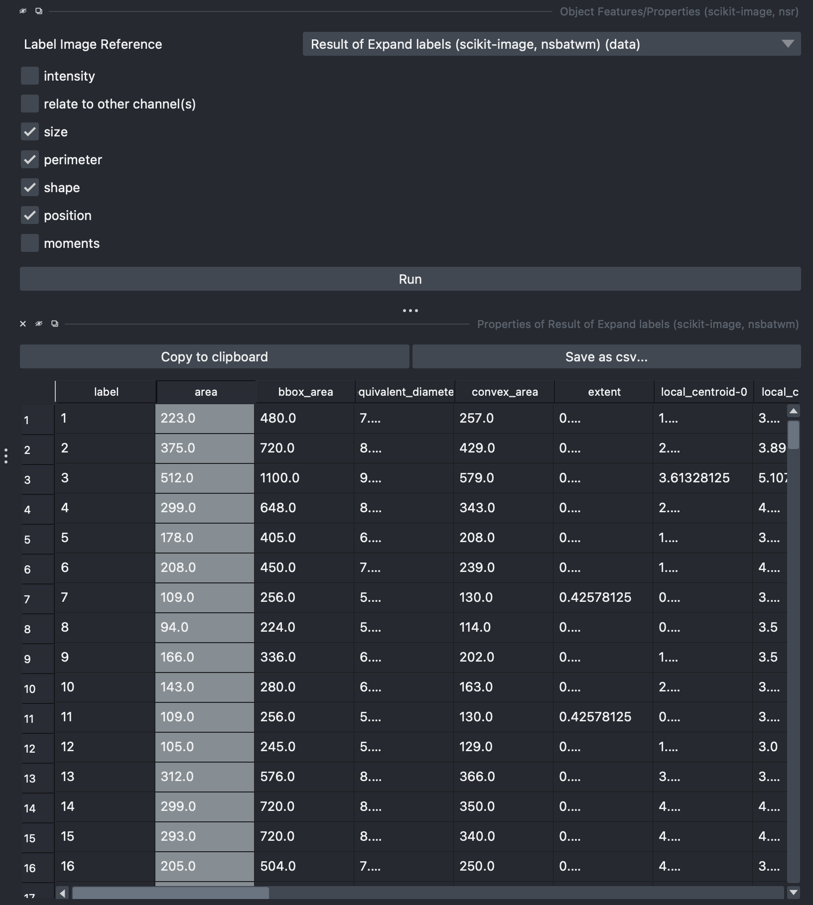
by double clicking any of the columns of this table, a new layer image will appear with colorcoded labels indicating the value of the selected measurement. Colormaps can be adjusted for preference.