Object-classification, dimensionality reduction and clustering
Object classification in Napari
Pixel classification, dimensionality reduction, and automatic clustering are common data-driven approaches used to analyze complex image data. Pixel classification assigns each pixel to a class based on its intensity or multi-channel feature values, enabling tasks such as segmentation or tissue labeling without explicit object detection. Dimensionality reduction methods (such as PCA, UMAP, or t-SNE) compress high-dimensional feature spaces into fewer dimensions while preserving key patterns or relationships, making large imaging datasets easier to visualize and interpret. Automatic clustering methods (e.g. k-means or similar algorithms) then group pixels or objects into clusters based on feature similarity, allowing unbiased identification of recurring patterns or phenotypes without predefined labels.
Learning Outcomes
By the end of this tutorial, participants will be able to:
- Train an object classifier with Napari
- Filter labels
- Extract morphological and intensity based parameters
- Plot parameters in 2D
- Apply a dimensionality reduction method
- Visualize the results
- Cluster subgroups of objects using K-means
These steps form a complete workflow: raw image → segmentation → cleanup → labeling → measurement → data viz
We’ll use Lund.tif as the example image https://zenodo.org/records/17986091
Requirements: - Everything you need is in the toml file in the Pixi/napari-devbio folder https://github.com/cuenca-mb/pixi-napari-devbio
–
0. Open the image and inspect the histogram
In the terminal, go to the directory Pixi/napari-devbio and run:
pixi run napari
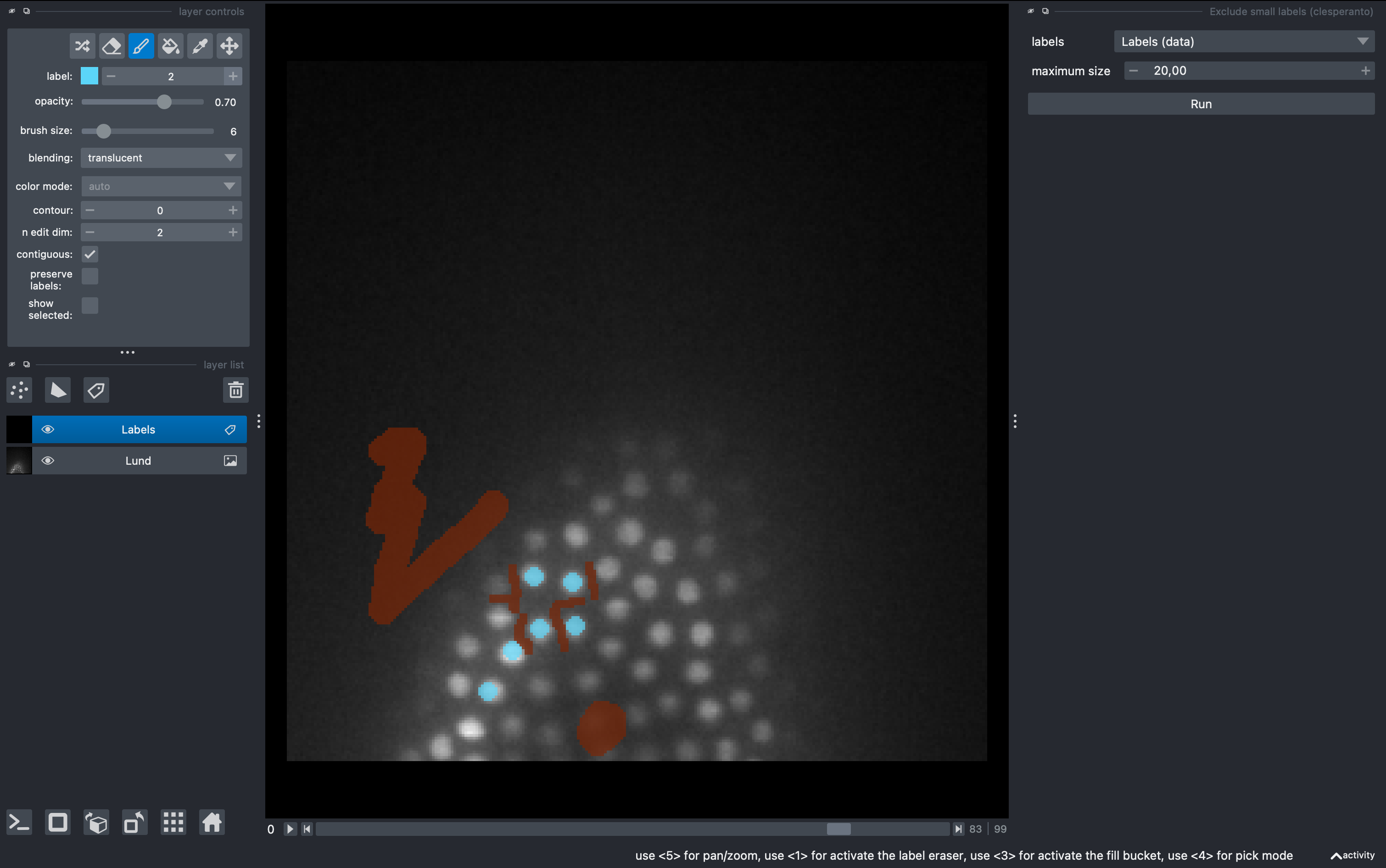
1. Open the image and create manual anotations
Drag and drop the file or
File → Open File
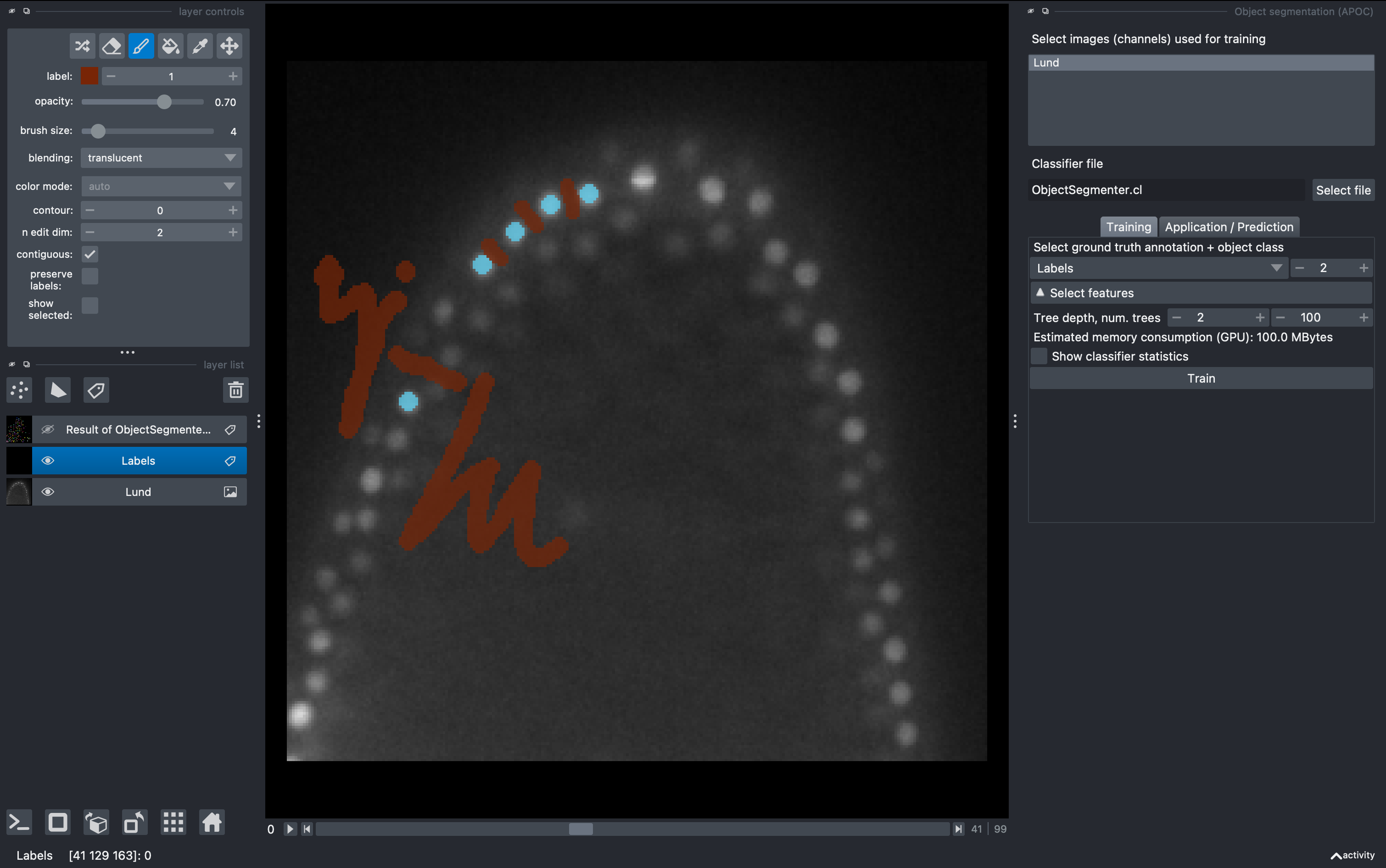
We will be able to see and explore the stack, and we can change to a 3D rendering with the option Toogle 2D/3D view in the lower left button pannel. We will create a labels layer to anotate some ground truth for our object classifier.
In the left pannel, select the brush tool and make some background anotations with the brush. Then change to label 2 and make some object annotations (cells).
2. Train the object classifier
Go to
Tools → Segmentation / labeling → Object segmentation (APOC)
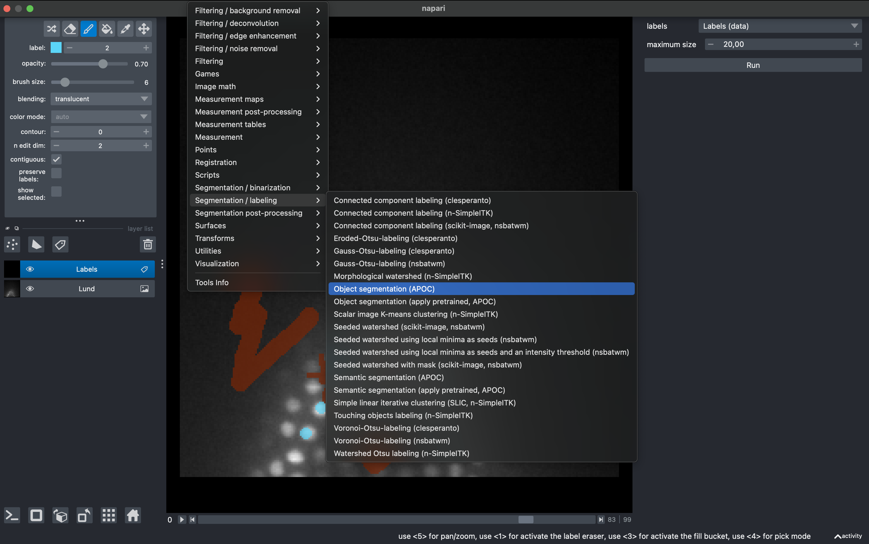
Select the raw data for training and the labels layer for ground truth. Then click Train. Observe the results in 3D. For better visualization you can hide the labels layer.
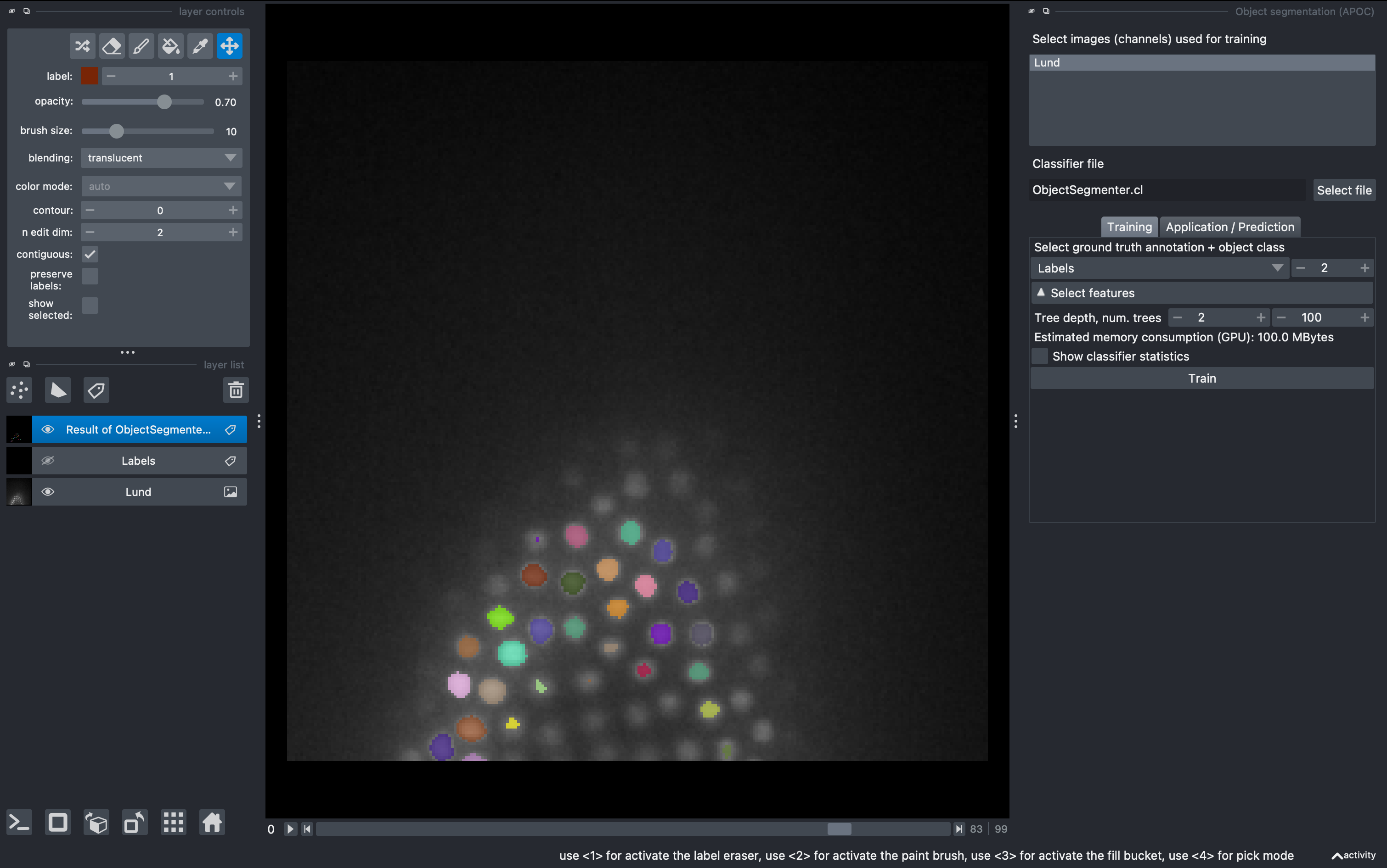
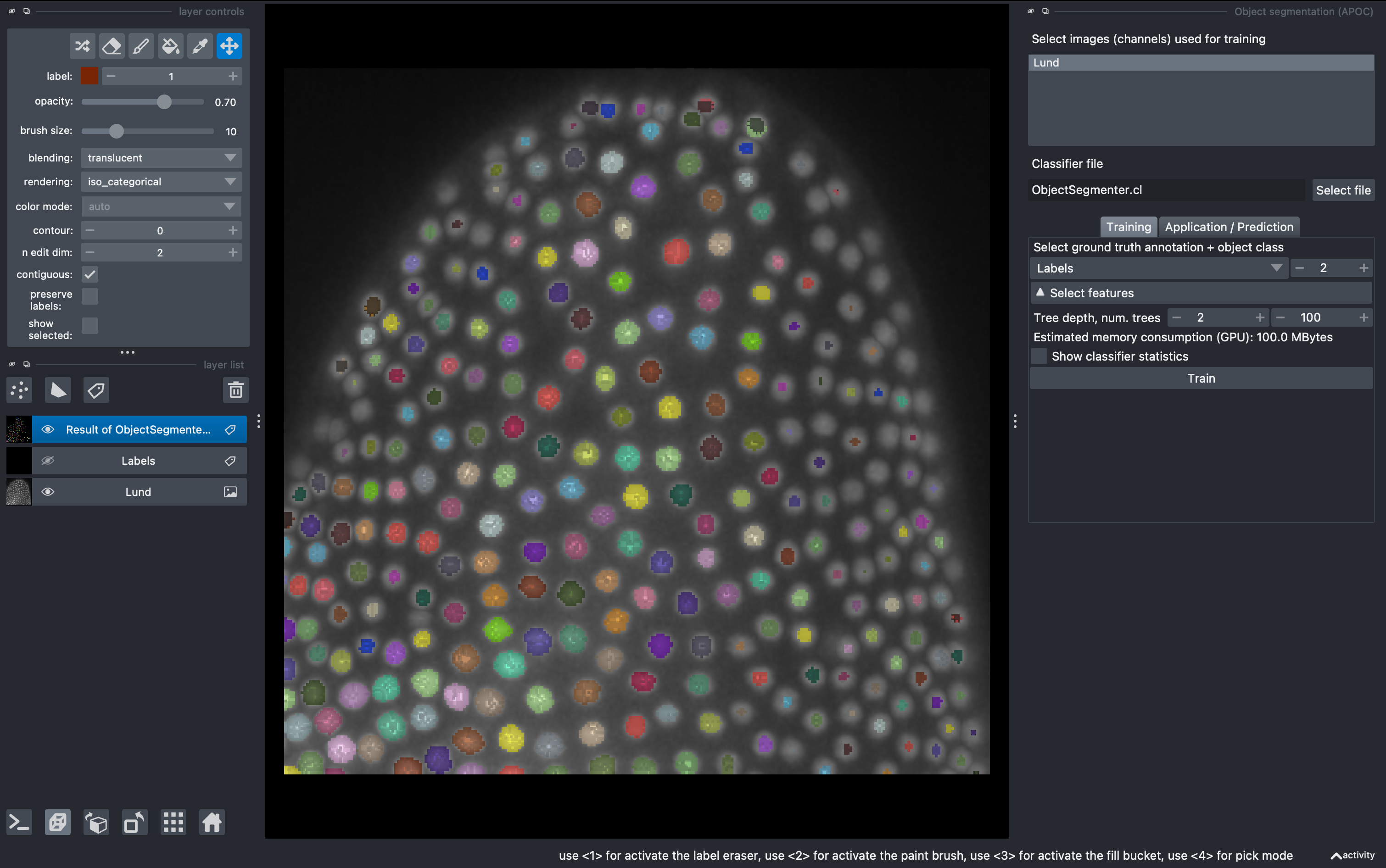
From this first round of training, very likely the result is not perfect. This is because our ground truth anotation was done on a single z slice, so the classifier will perform well only around that depth. We can do several rounds of training.
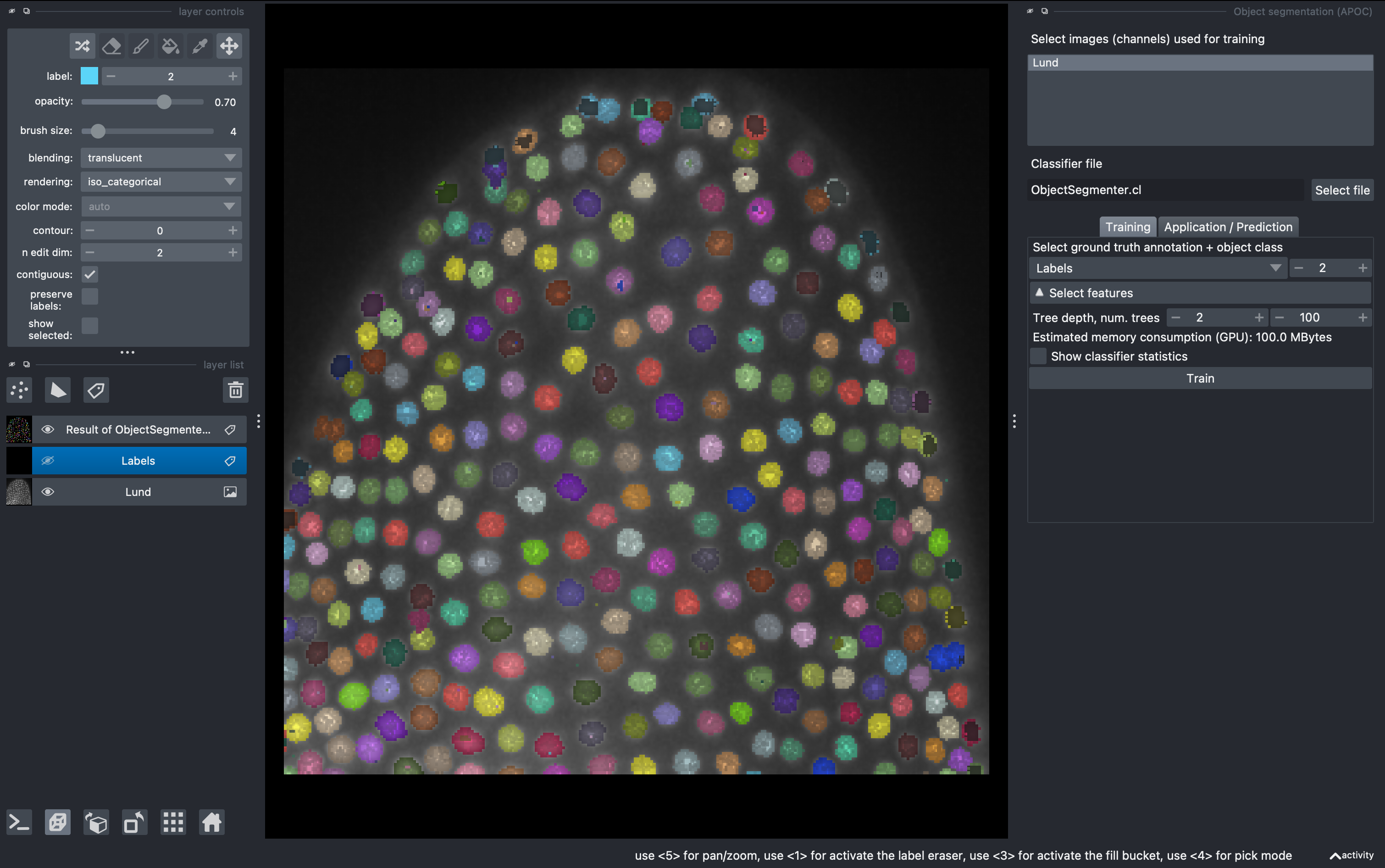
Select again the labels image, and in the 2D mode go to a different z. Perform new anotations, preserving the label orders for background and object. Then just click Train again and observe the new results. Repeat as needed. Note that a classifier file will be produced and overwritten after each training. This can be used for batch segmentation of data from the same experiment/microscope.
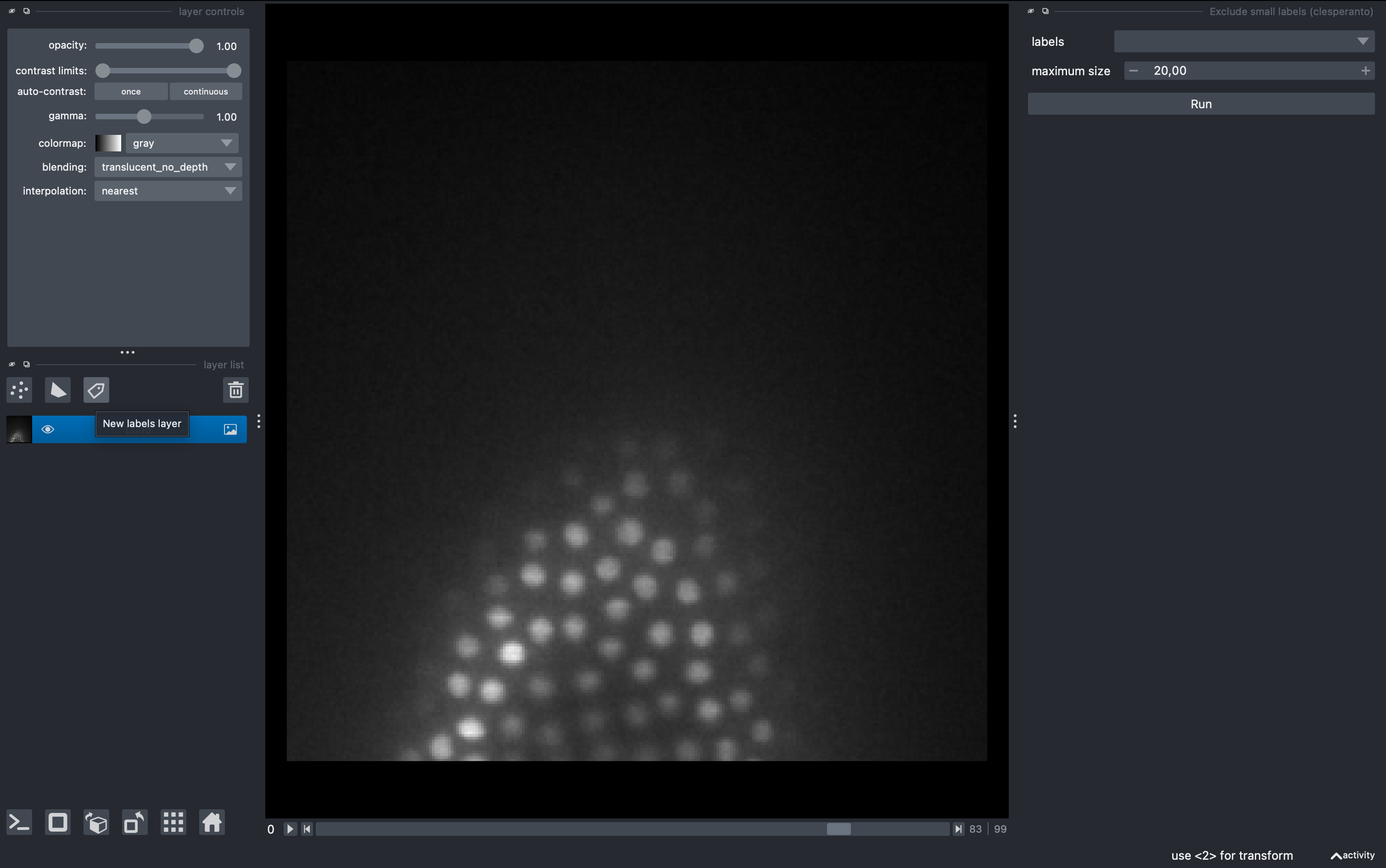
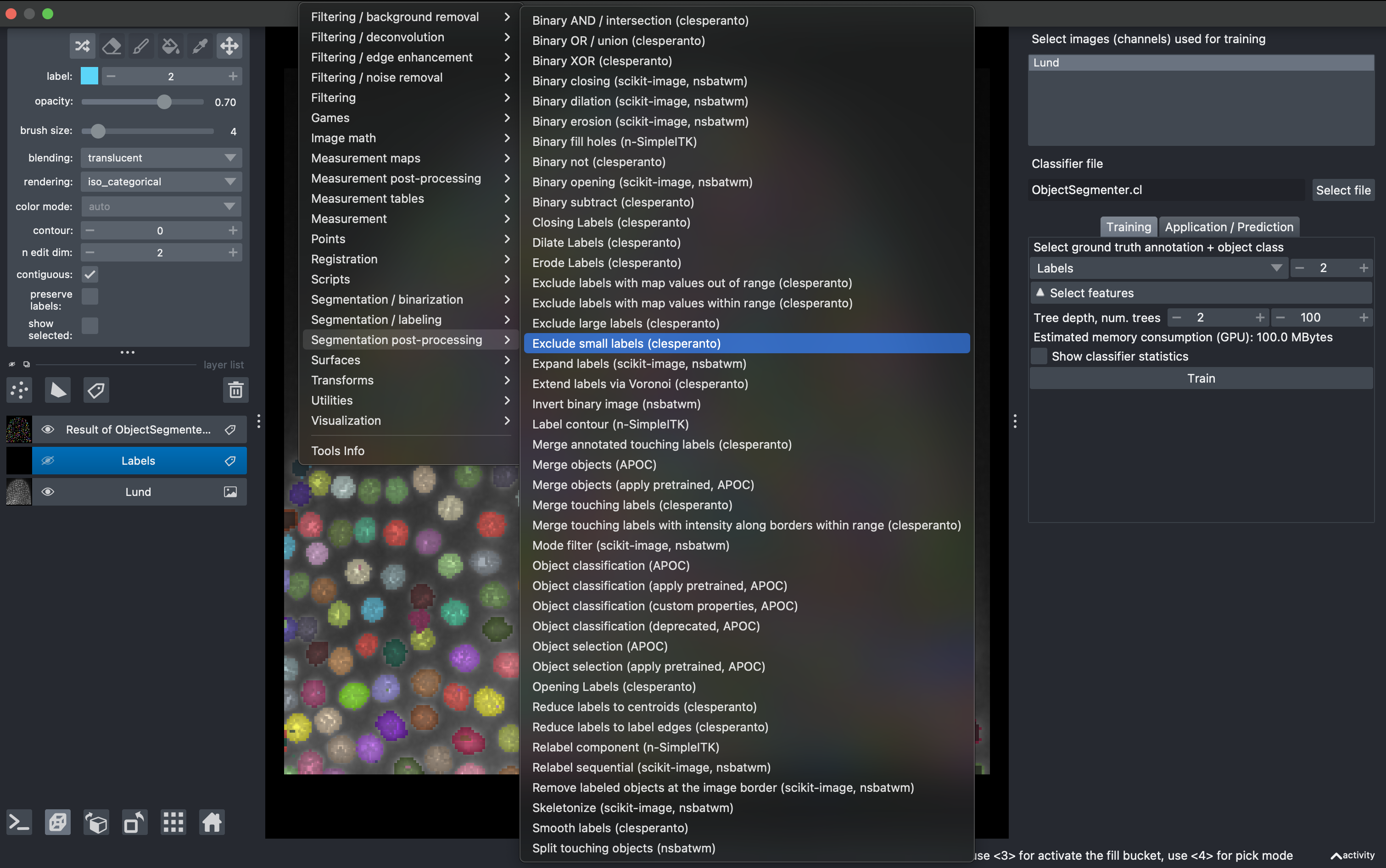
3. Filter small objects and quantify parameters
Now there might be some small objects that we want to filter. Go to
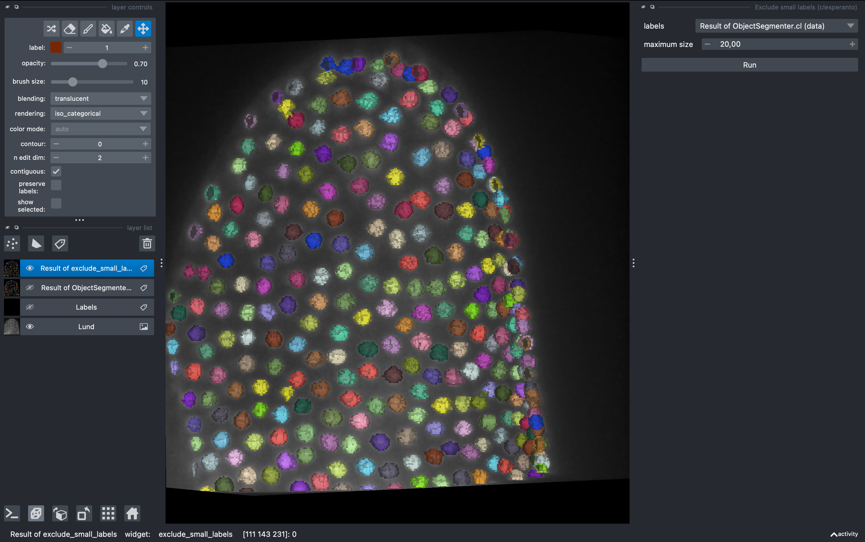
Tools → Segmentation post-processing → Exclude small labels
Then select the layer Result of ObjectSegmentation and impose a minimum size of 20 (it will say maximum size in napari, but it is a mistake from the developers). Run it and observe the final labels (hide the old labels for better visualization.
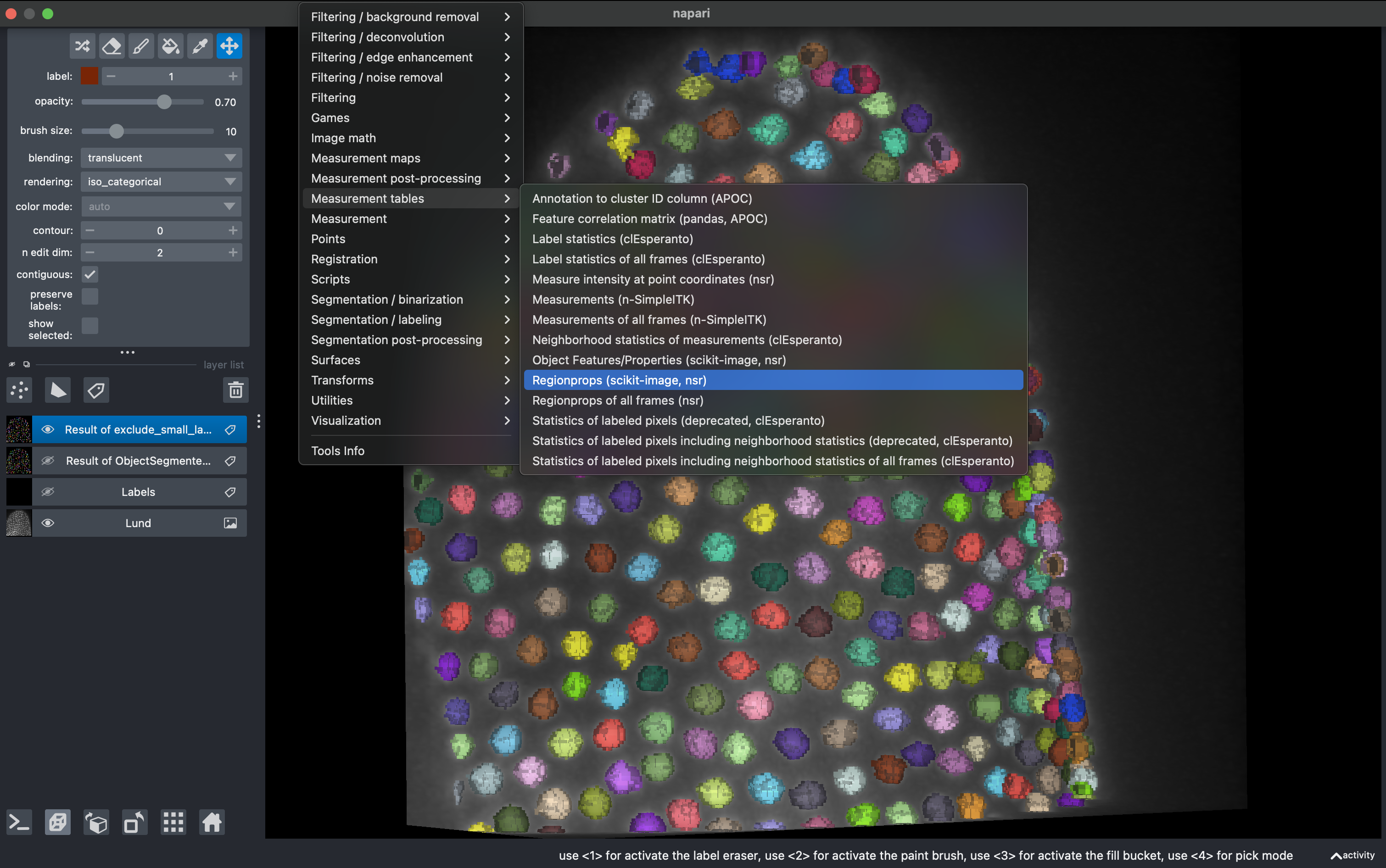
Now that we have a nice set of labels in 3D, we will quantify intensity and morphology based parameters for further analysis.
Go to
Tools → Measurement tables → Regionprops
Select all parameters except moments and click run.
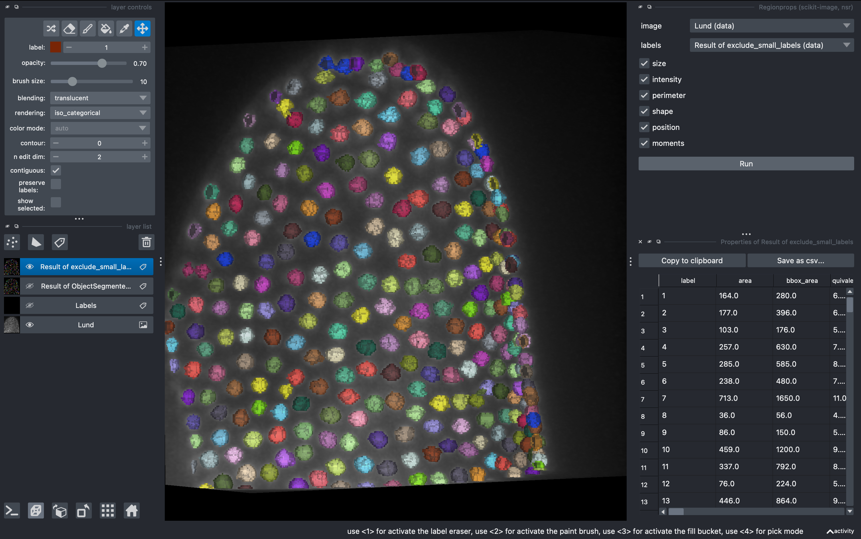
We can export this table or visualize some of the data using the cluster plotter.
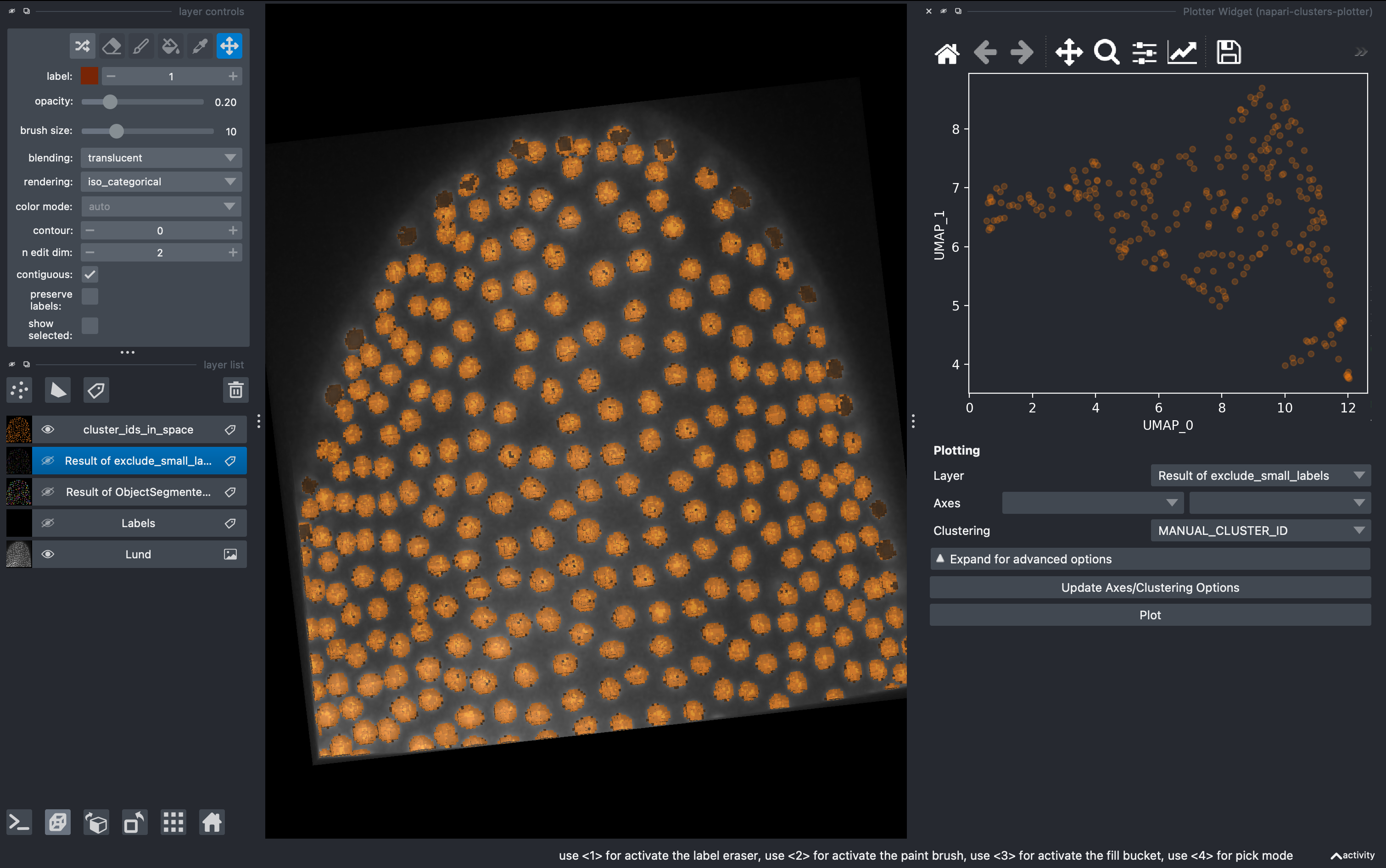
4. Data visualization with clusters plotter
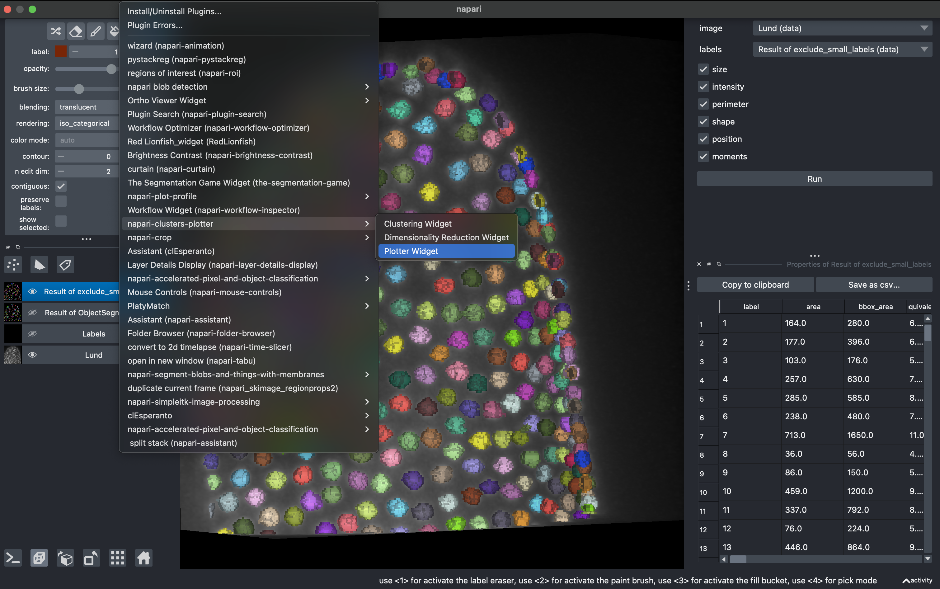
Go to
Plugins → napari-clusters-plotter → Plotter widget
In here you can select any measurement (column) from the region props table and make scatter plots.
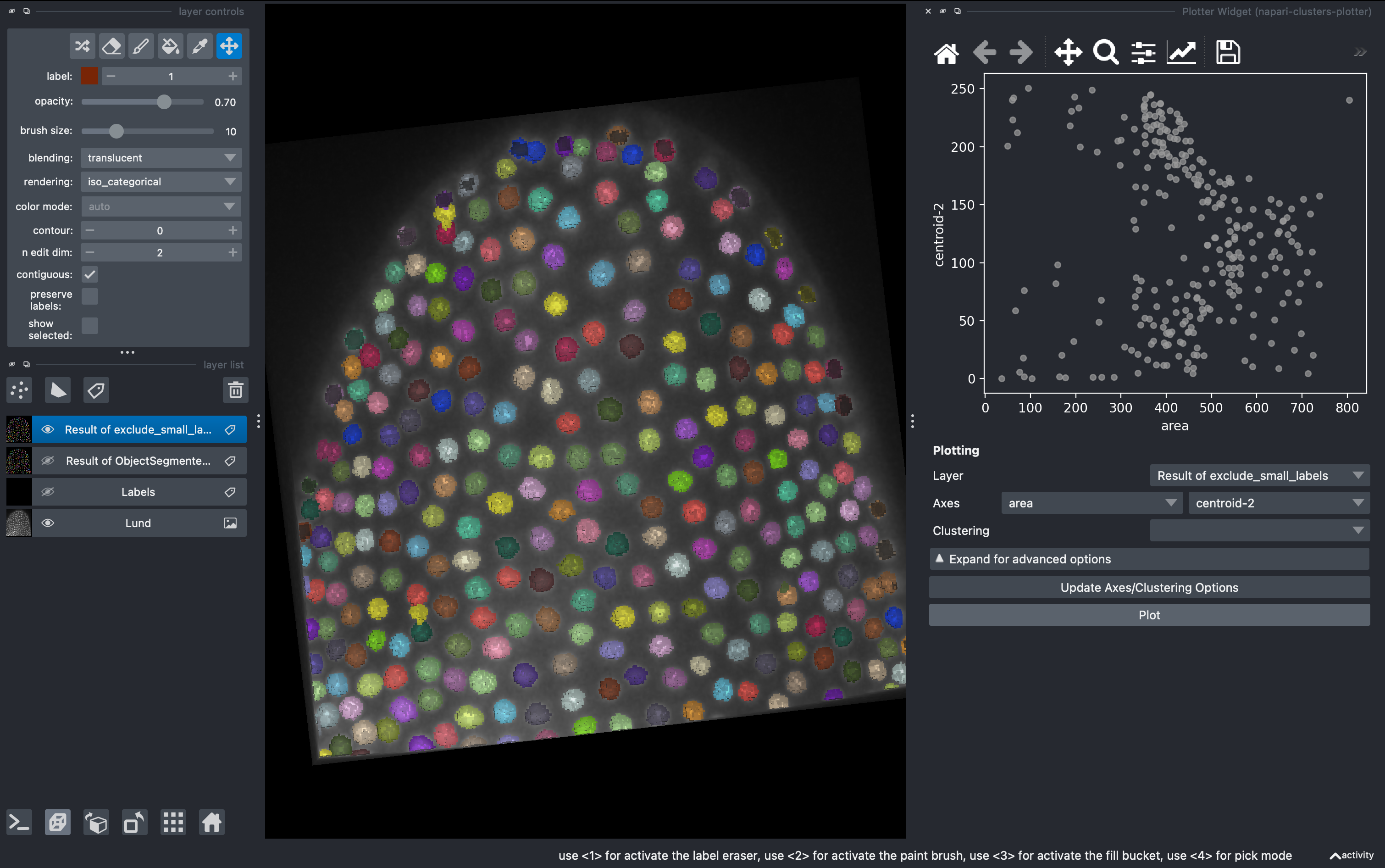
A very useful tool is that we can draw in the plot closed curves and the objects falling inside will be automatically colorcoded and visualized in the 3D rendered image. I recommend hiding all the other layers except the raw image.
By pressing shift, we can draw further subgroups.

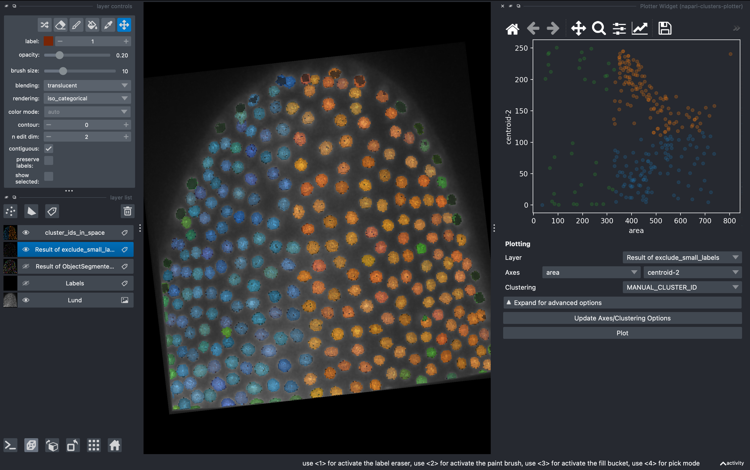
This manual selection generates a new column in the regionprops table with the identifier for us to export and further analyse in other software.
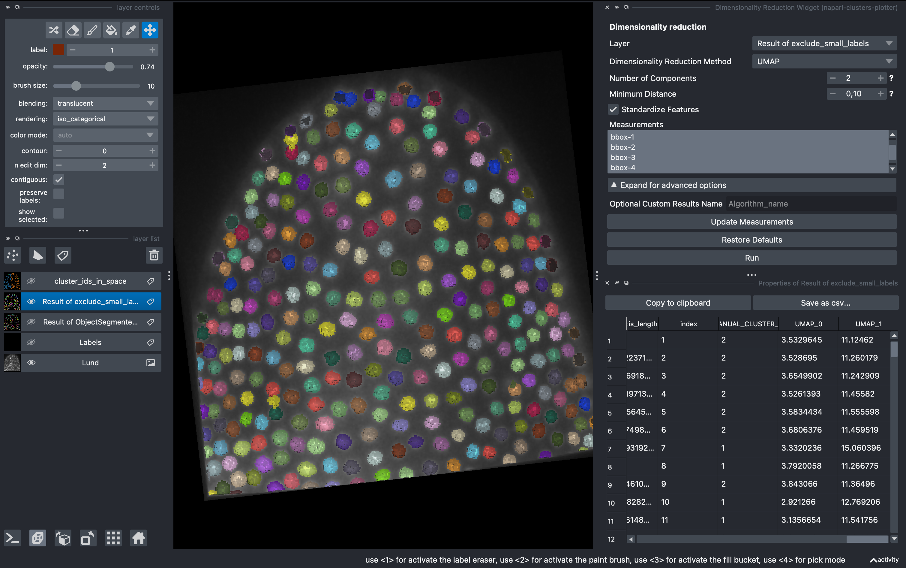
5. Dimensionality reduction
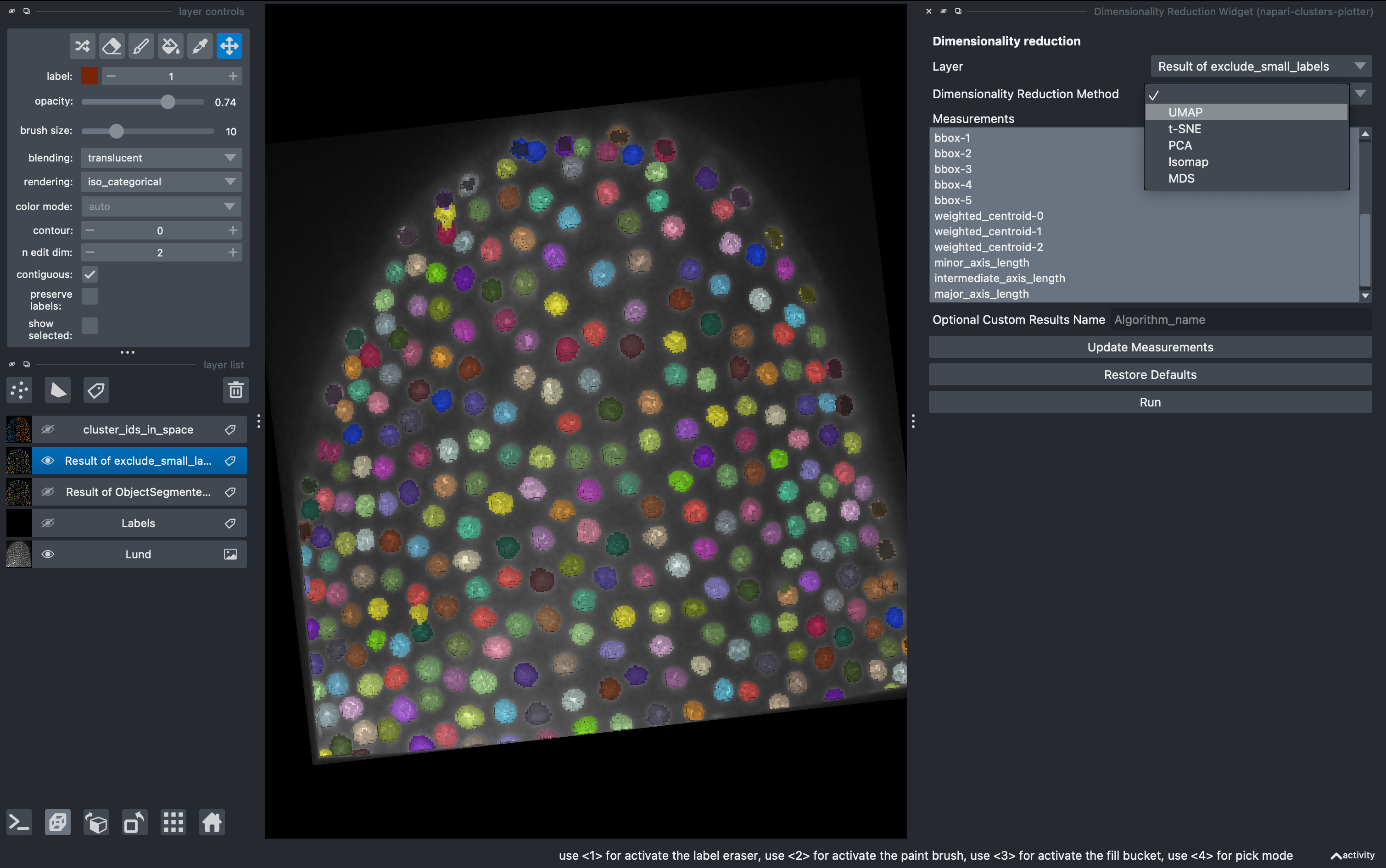
Go to
Plugins → napari-clusters-plotter → Dimensionality Reduction Widget
This is a very useful tool in which we can apply a variety of dimensionality reduction methods to our list of parameters. In this example I used UMAPS. We can select how many components we want and after hitting run they will be added to our regionprops table.
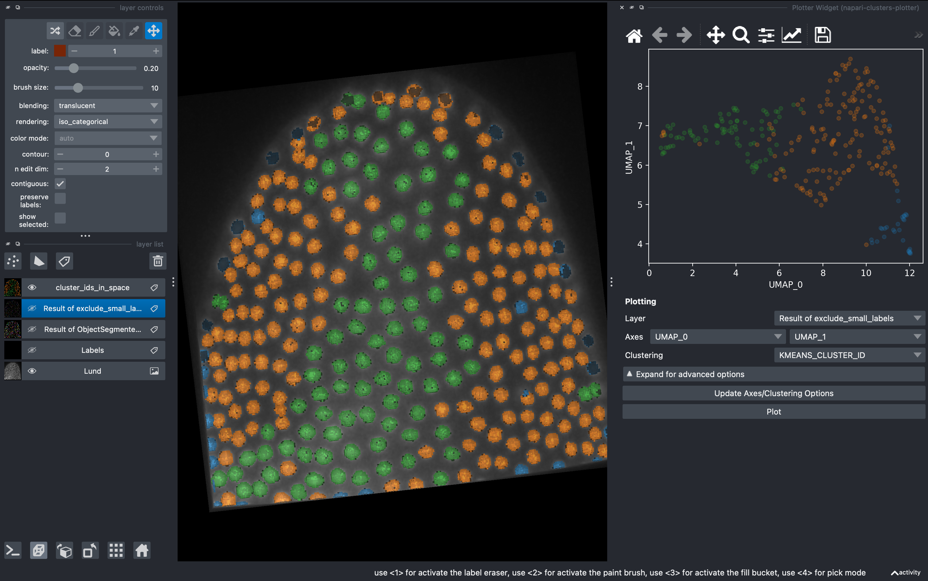
After doing this, we can come back to the Plotter Widget and plot this two components of the UMAP and generate more complex clustering of the data manually.
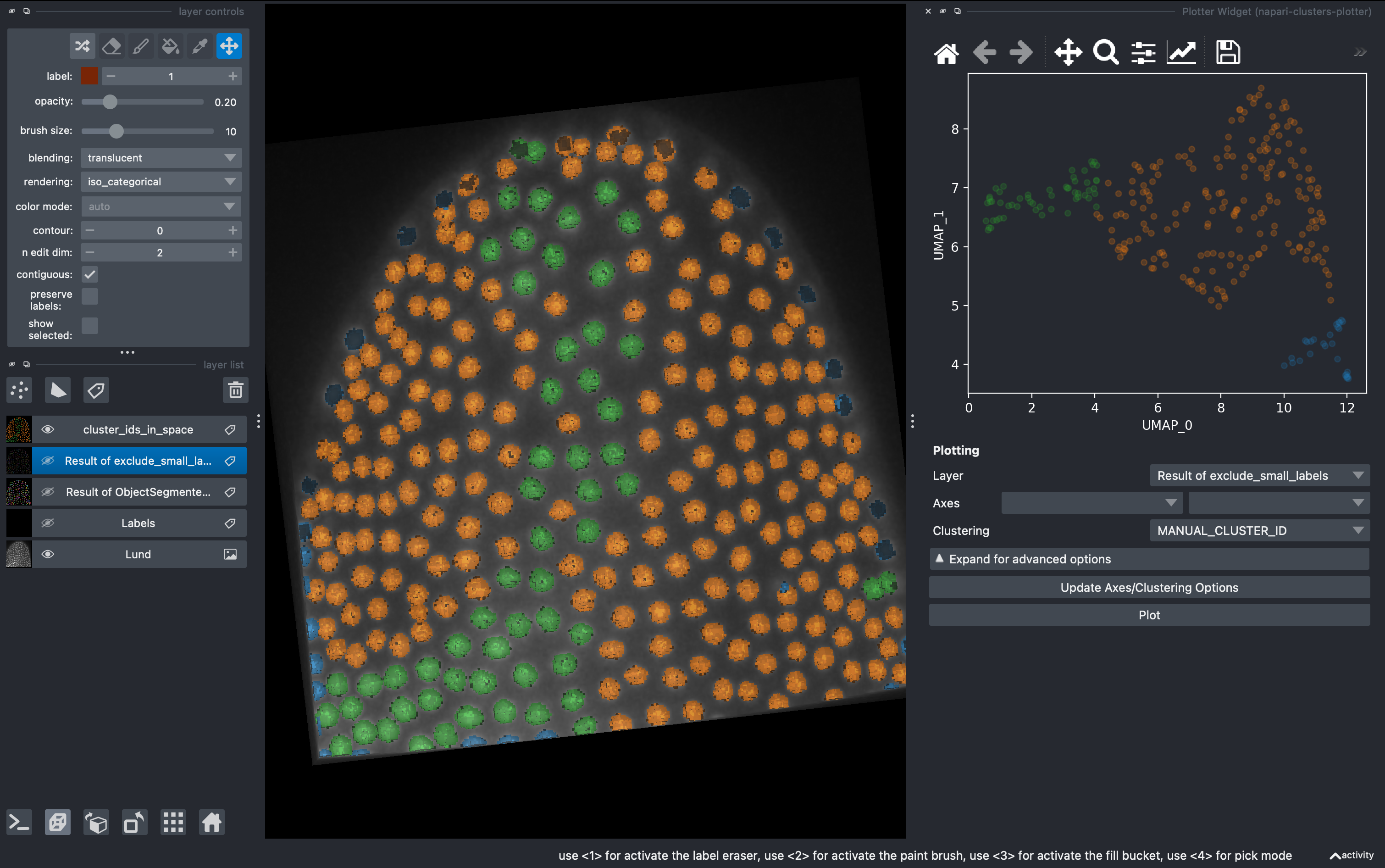
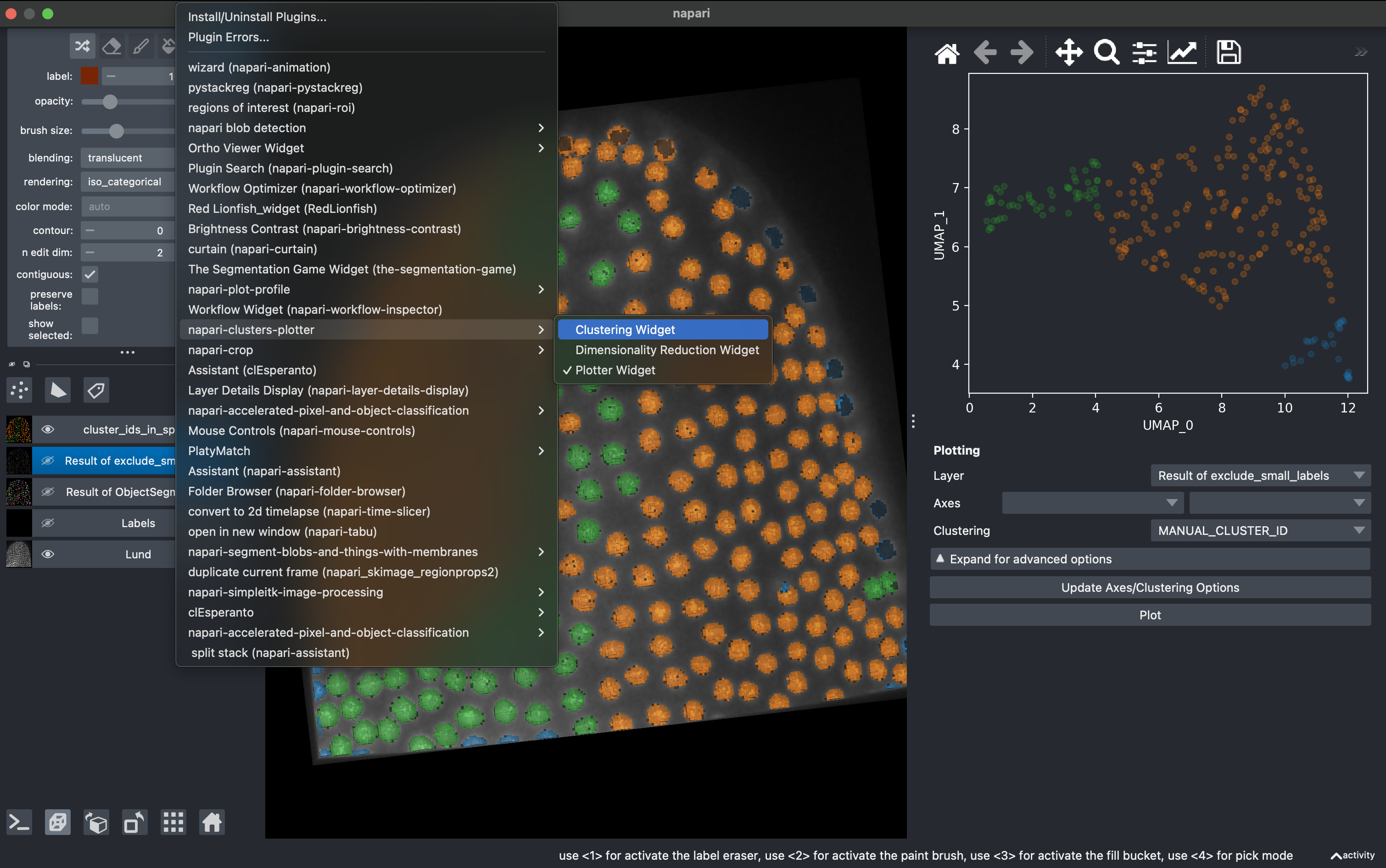
6. Unsupervised clustering
But what if we don’t want to be biased when clustering the data in subgroups? We can use unsupervised methods includded in this plugin. Go to
Plugins → napari-clusters-plotter → Clustering Widget
Select the K-MEANS method, impose 3 clusters and run. This will generate a new column with the cluster ID for each object.
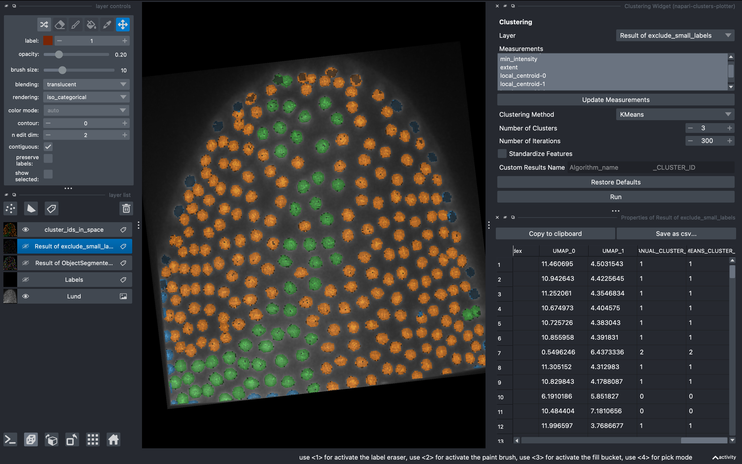
Now going back to the Plotter Widget, we can select the UMAP axis AND the K-MEAN cluster IDs to automatically colorcode the objects belonging to different classes.