Multiview reconstruction using BigStitcher

Summary

Multiview reconstruction is the process of registering and fusing microscopy data acquired from multiple angles into a single, isotropic stack.

This tutorial shows how to register and fuse multiview lightsheet microscopy datasets using the plugin BigStitcher (Preibisch et al. 2010; Hörl et al. 2019) in Fiji (Schindelin et al. 2012).

We will cover how to convert the raw data for visualization in the BigDataViewer (Pietzsch et al. 2015), how to best detect interests points for registration, the different approaches to register views, and how to fuse the views to reconstruct an isotropic dataset.

Requirements

• Fiji (Schindelin et al. 2012)
• BigStitcher plugin (Preibisch et al. 2010; Hörl et al. 2019)
• Fly Embryo Multiview Lightsheet dataset (Vellutini 2025)

Setup

Install Fiji

• Go to https://fiji.sc, choose Distribution: Stable, and click the download button.
• Copy the downloaded archive to your working directory and unzip it.

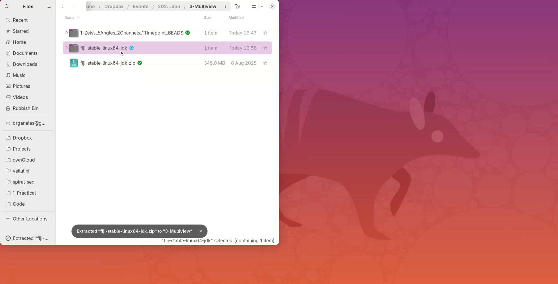
• Open the Fiji.app directory and double-click on the launcher.

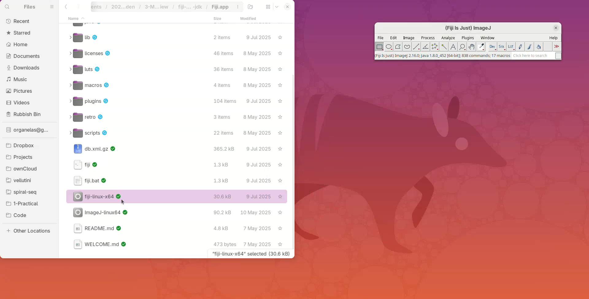
The main window of Fiji will open.

Install BigStitcher

• Click on Help > Update....

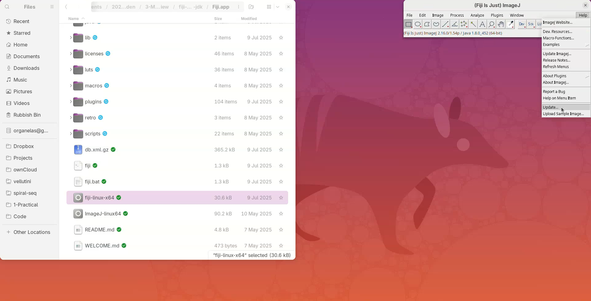
The updater will run and say if Fiji is up-to-date.

• Click on Manage Update Sites.

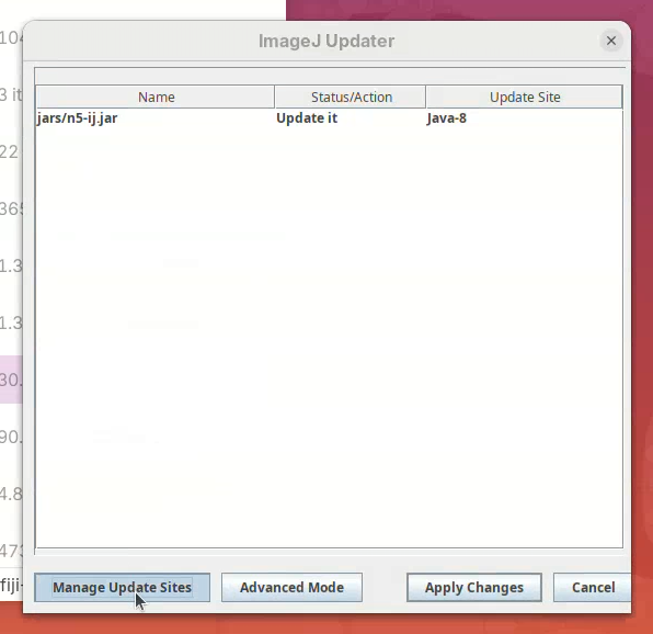
A window will open with a list of plugins available to install in Fiji.

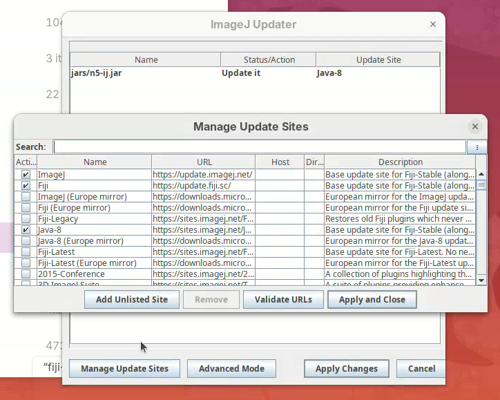
• Find BigStitcher in the list and click on the checkbox and Apply and Close.

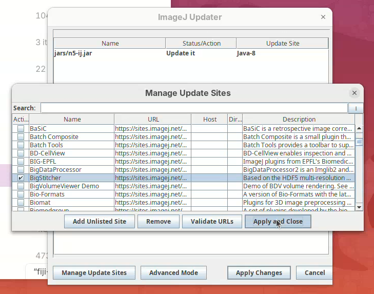
• Then click on Apply Changes.

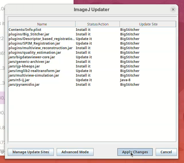
• Wait… until the downloads are finished. Then, click OK.

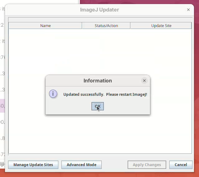
• Restart Fiji (close window and double-click the launcher).
• Check if BigStitcher is installed under Plugins > BigStitcher.

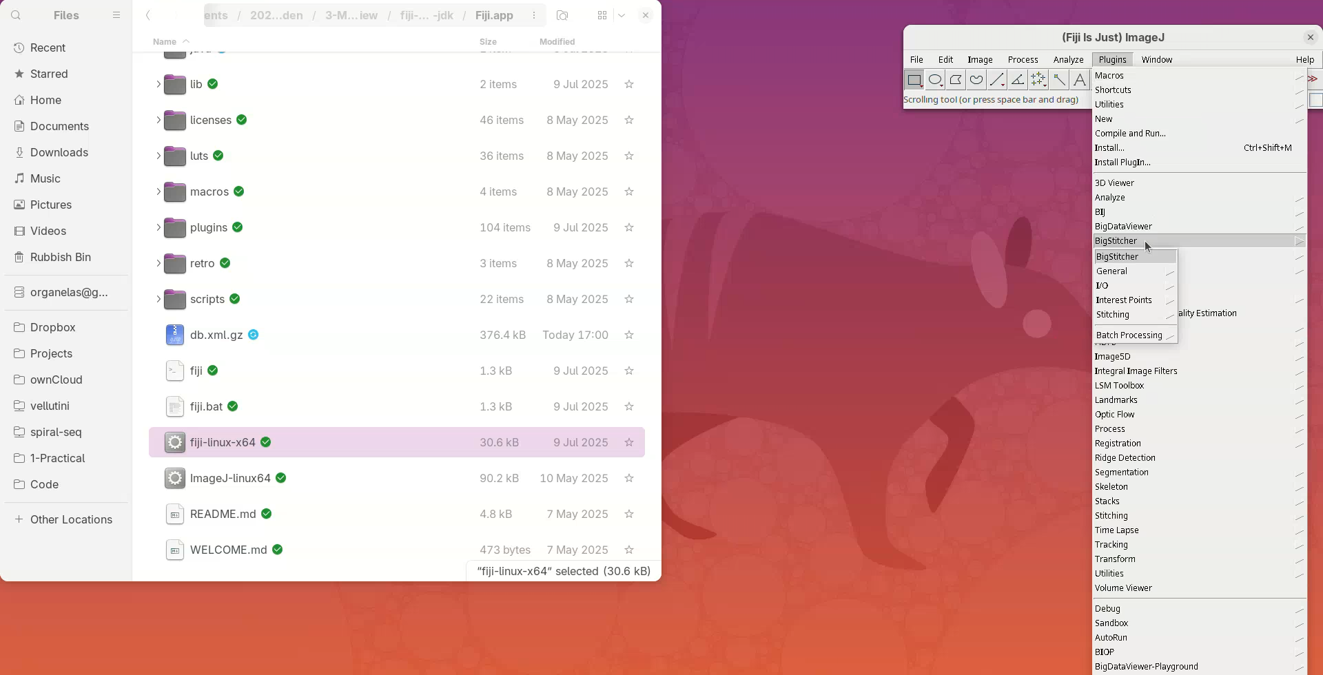
Fiji and BigStitcher are ready!

Download dataset

• Dmel_btd-gap_1tp_5v_2c_beads.czi dataset from this Zenodo repository (Vellutini 2025). The direct link to the file is here (3.2GB).

Inspect dataset

The dataset is a single CZI file that contains a single timepoint with 5 different views, each view with 2 channels and 60 slices. The XY resolution is 0.276 µm and the Z resolution is 3 µm. The dataset has fluorescent beads around the sample, which we will use to register the views.

Let’s inspect the dataset in Fiji.

Open file

• Drag and drop the CZI file in Fiji’s main window.

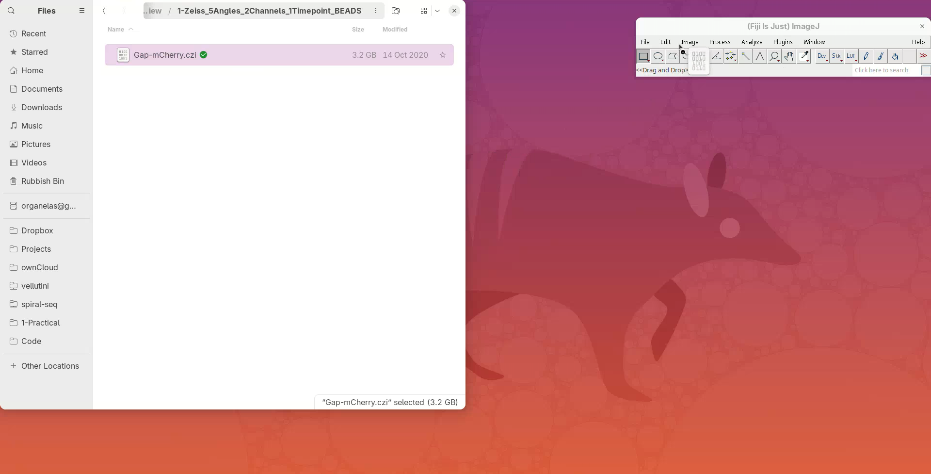
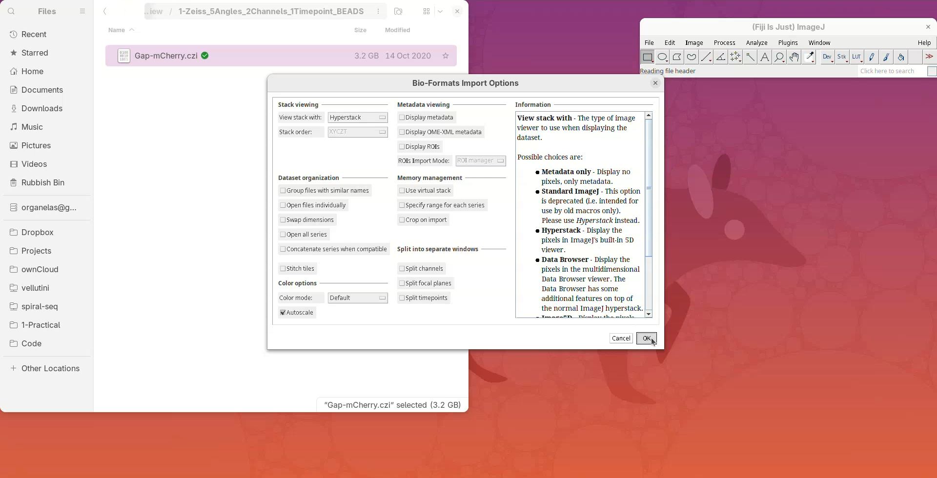
A Bio-Formats Import Options window should open. That’s the default importer for proprietary file formats with many options, but for now we go with the default.

• Press OK.

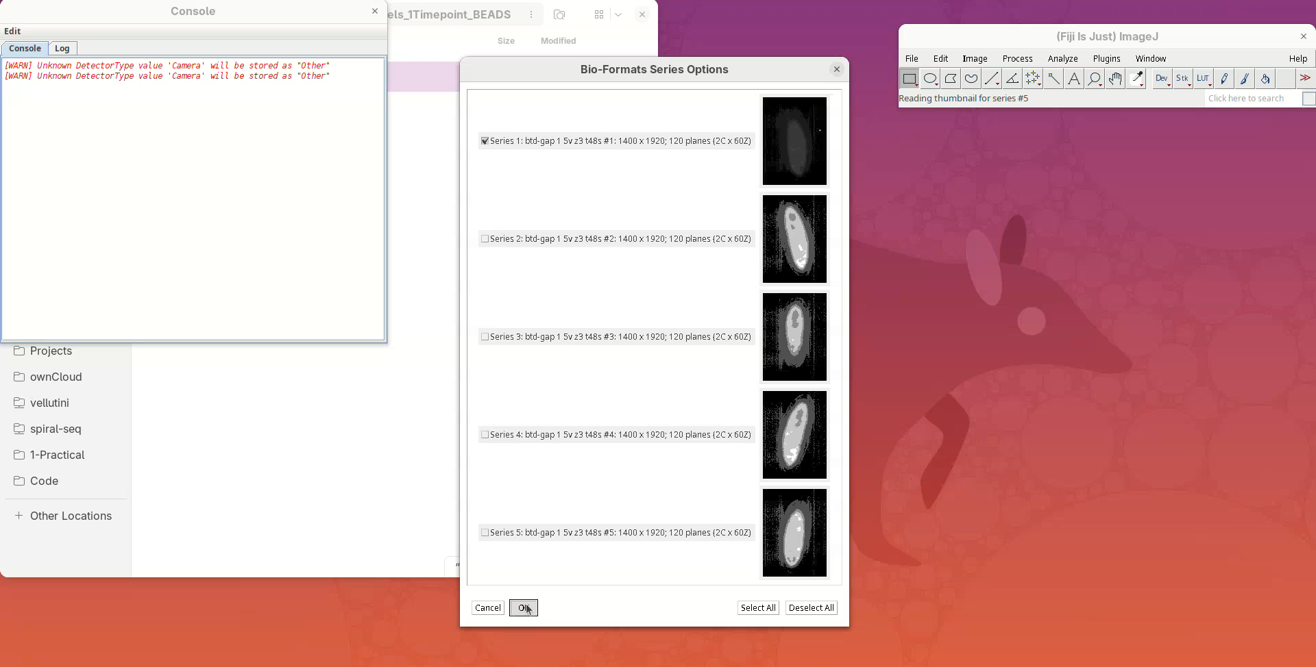
A Bio-Formats Series Options window will open. Bio-Formats recognized that this file contains more than one view (series) and is asking which ones do we want to open. We just want to inspect the first view since they will be quite similar.

• Press OK.

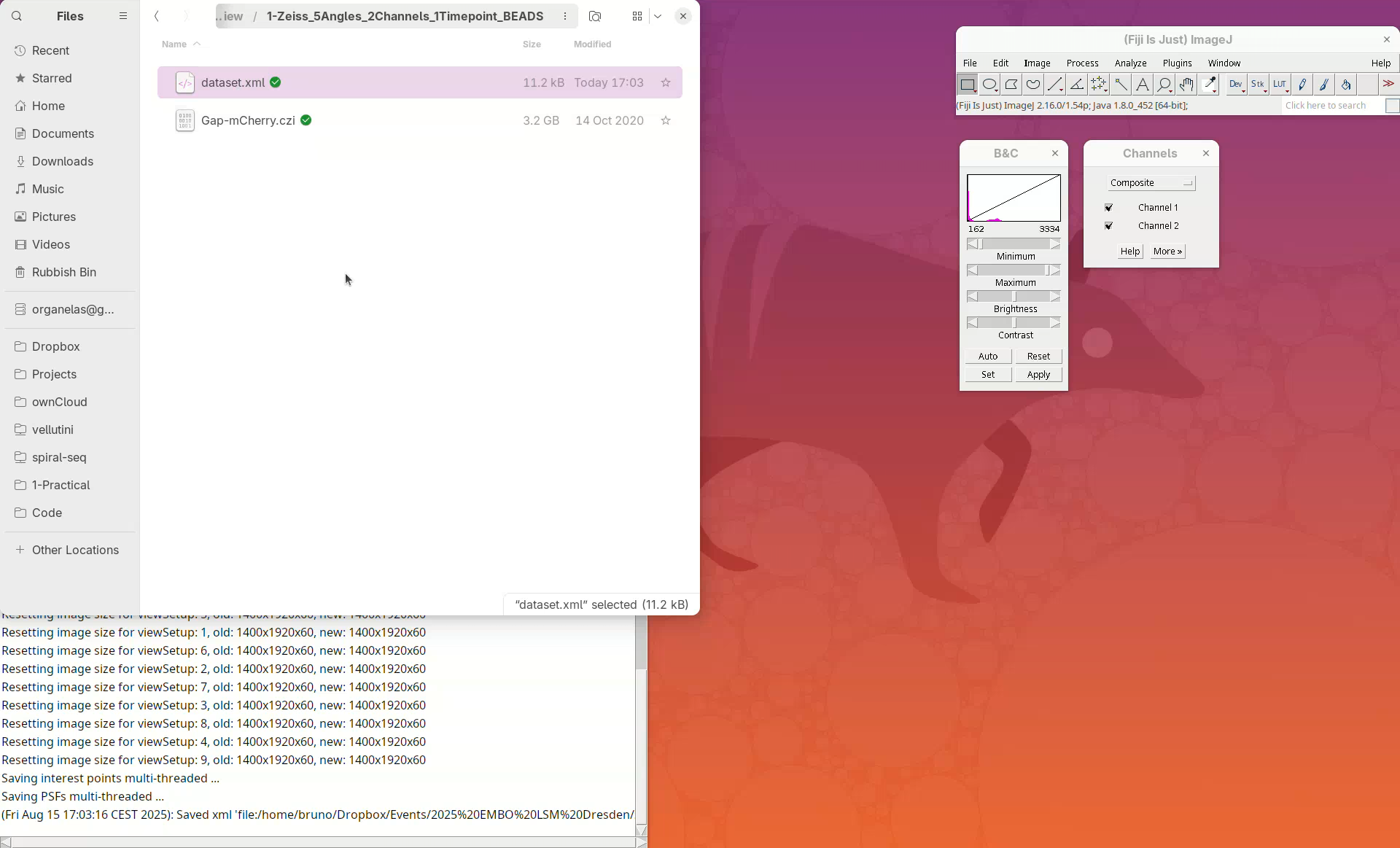
Adjust contrast

A big window with a black background will open.

• Check if the dimensions were correctly assigned (information line at the top and sliders at the bottom).

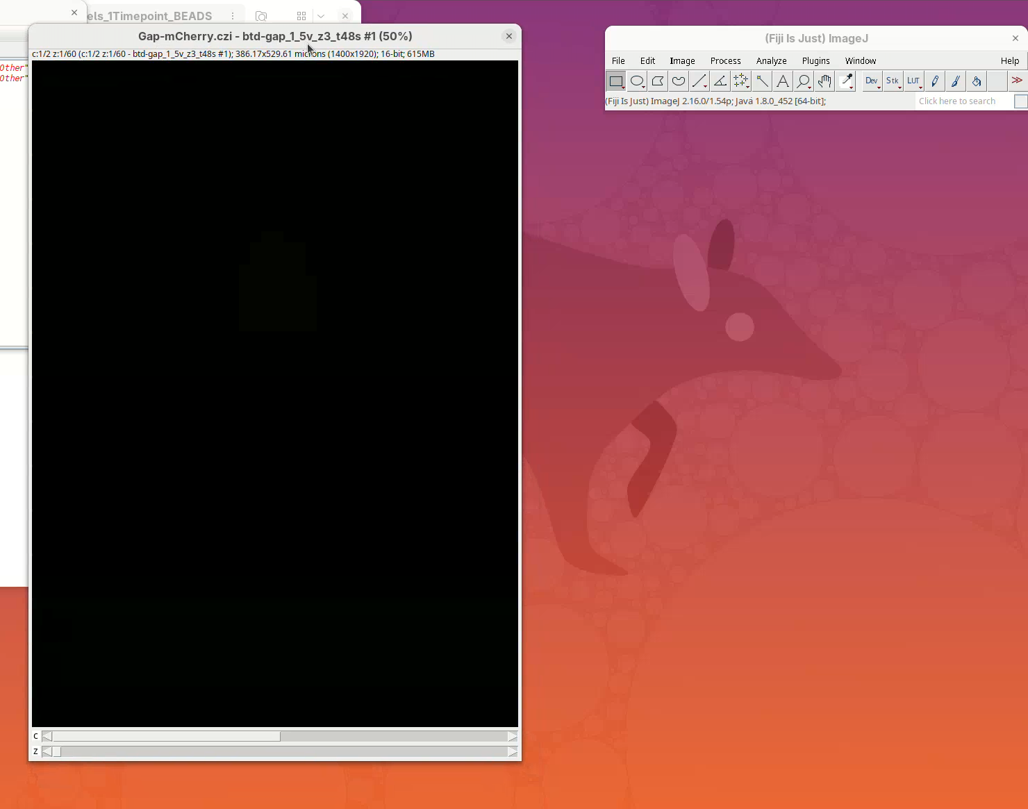
To see something, we first need to adjust the levels.

• Open the Brightness/Contrast (B&C) tool with Image > Adjust > Brightness/Contrast... (or Ctrl+Shift+C) and the Channels Tool with Image > Color > Channels Tool... (or Ctrl+Shift+Z).

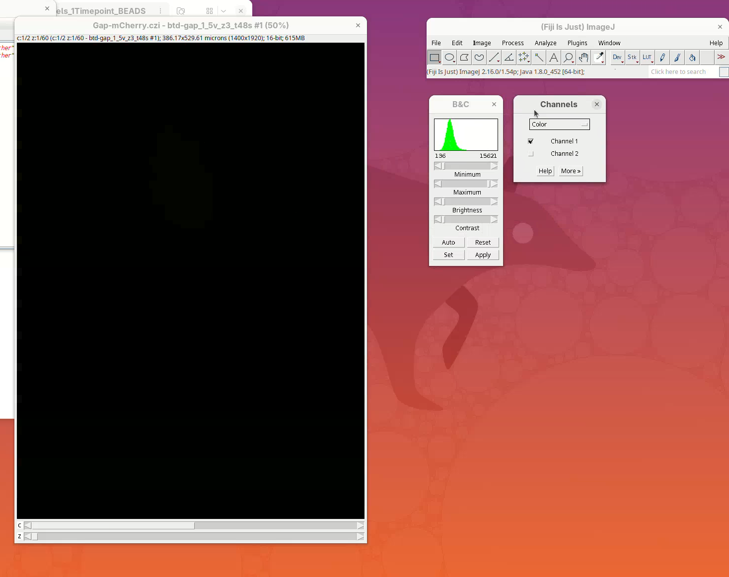
• Press Reset to adjust the levels of Channel 1 then slide the Z position to the middle of the sample and press Reset again.

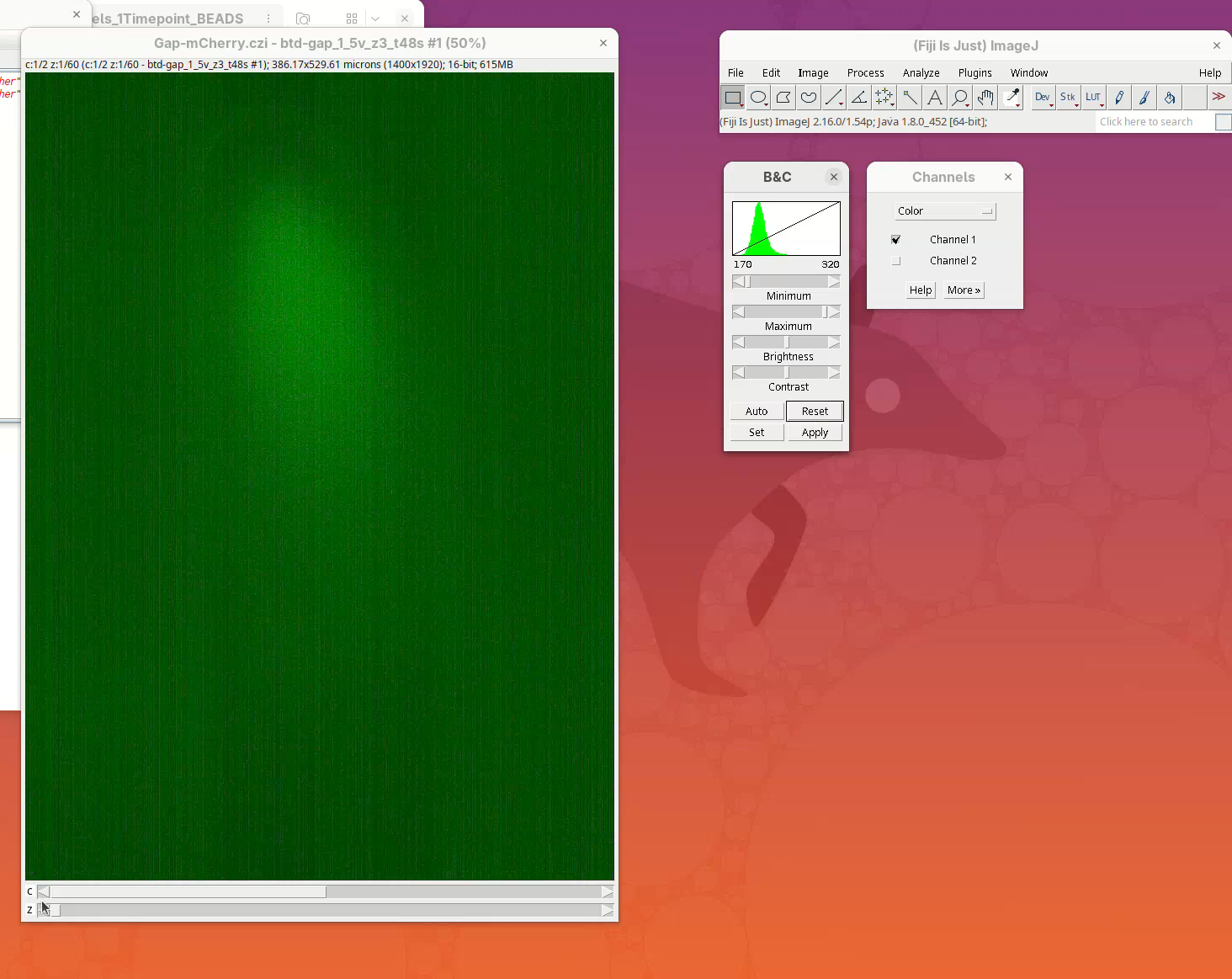
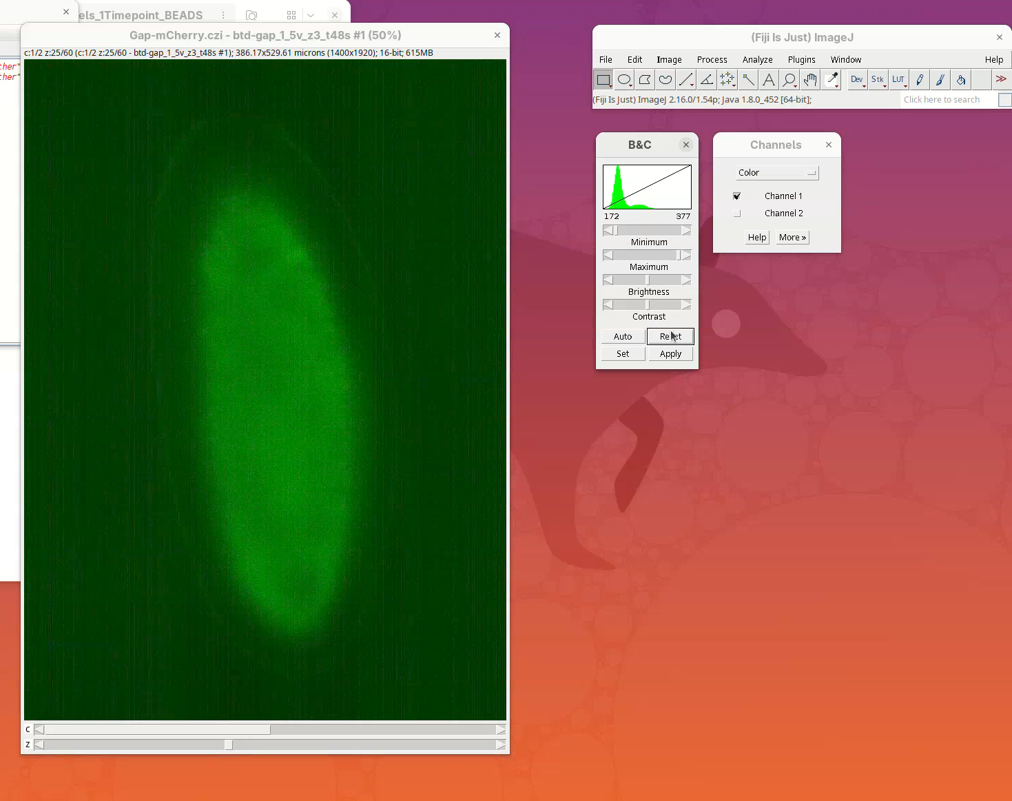
• Now move the Channel slider to Channel 2 and press Reset.

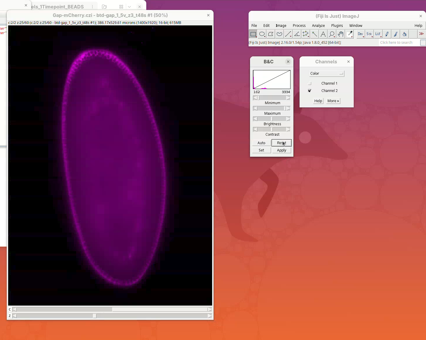
• In the Channels window, change the menu Color to Composite.

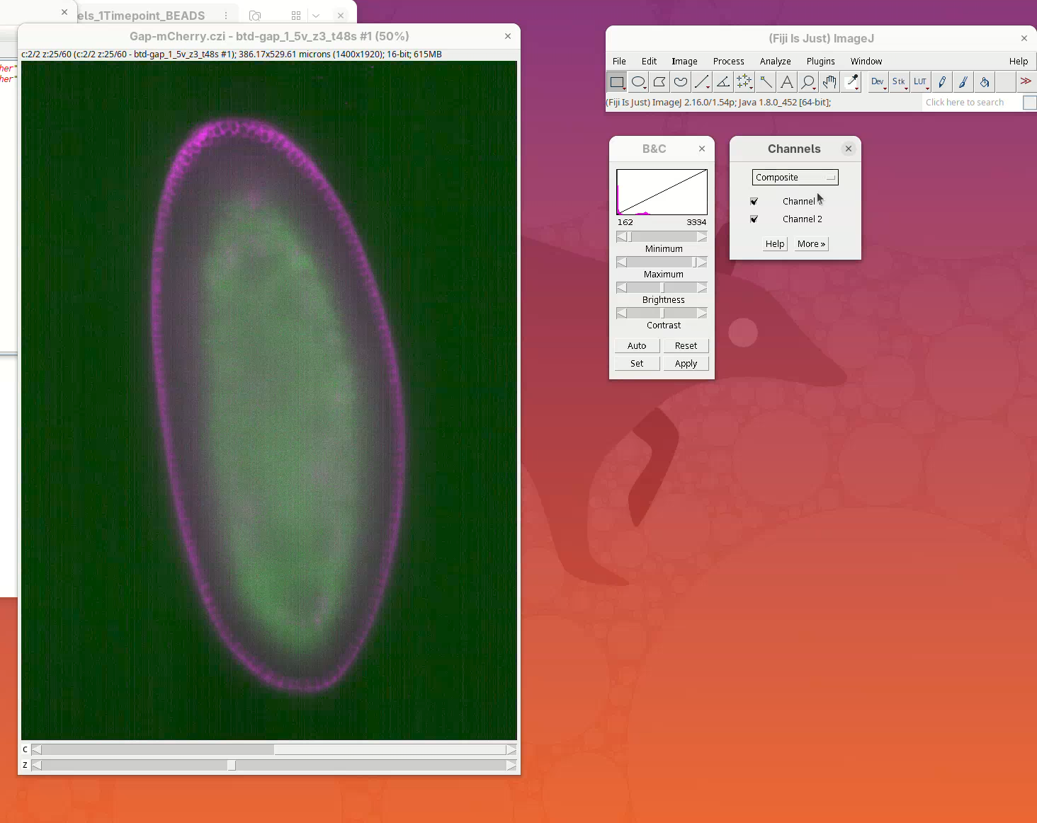
The sample is ready to be visualized.

Open orthogonal views

To get a sense of the data tridimensionality we want to look at the XY, XZ, and YZ optical sections.

• Click on Image > Stacks > Orthogonal Views (or Ctrl+Shift+H). It takes a moment; XZ and YZ panels will open.

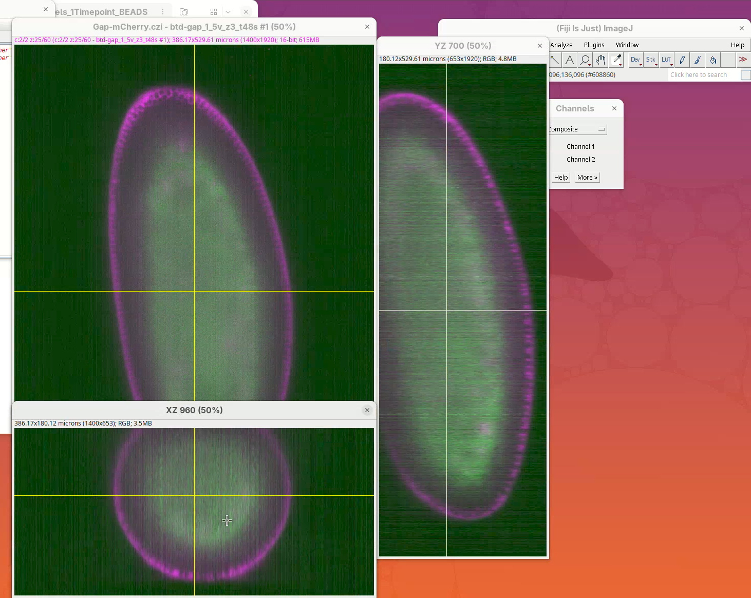
• Resize the main window to fit the screen.

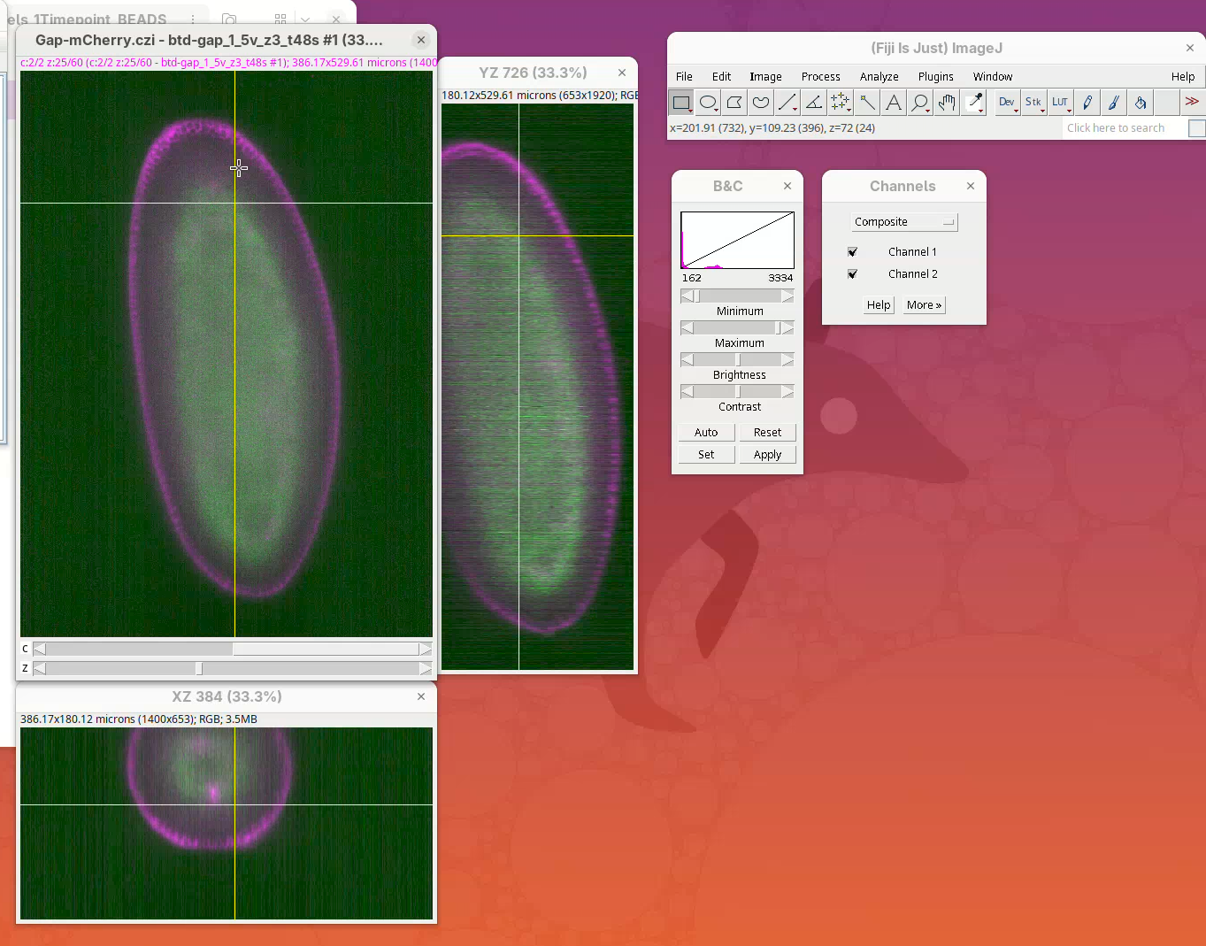
The sample is a fly embryo which resembles a cylinder in 3D.

• Explore the dataset by clicking and sliding the mouse pointer through the different images.
• When done, close the stack.

Define dataset

Before we begin, we need to define a multiview dataset and resave the dataset. Defining a multiview dataset will create an XML file where all the dataset metadata and information and data from the registration process will be stored.

• Go to Plugins > BigStitcher > General > Define Multi-View Dataset.

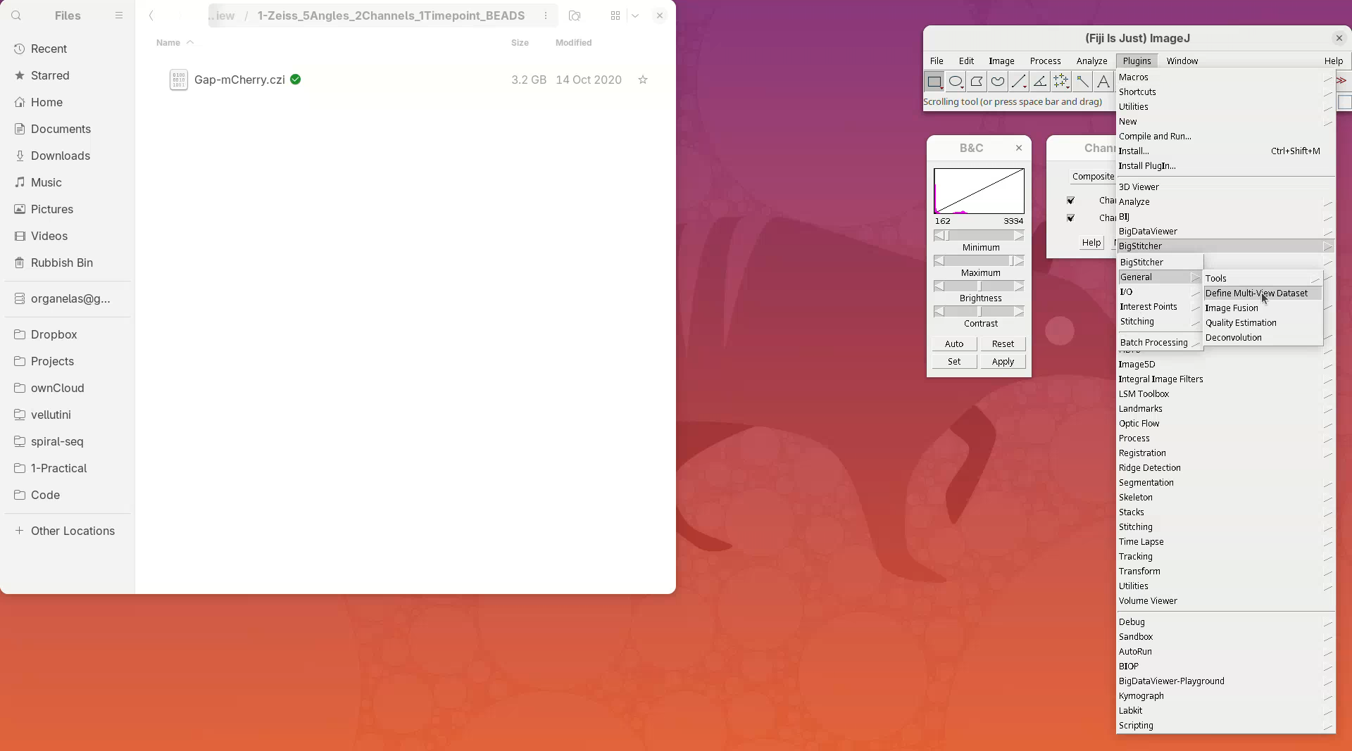
A window named Choose method to define dataset will open.

• On the Define Dataset field choose Zeiss Lightsheet Z.1 Dataset Loader (Bioformats) from the dropdown menu, since our testing dataset is from Zeiss Lightsheet Z.1.
• Then, press OK.

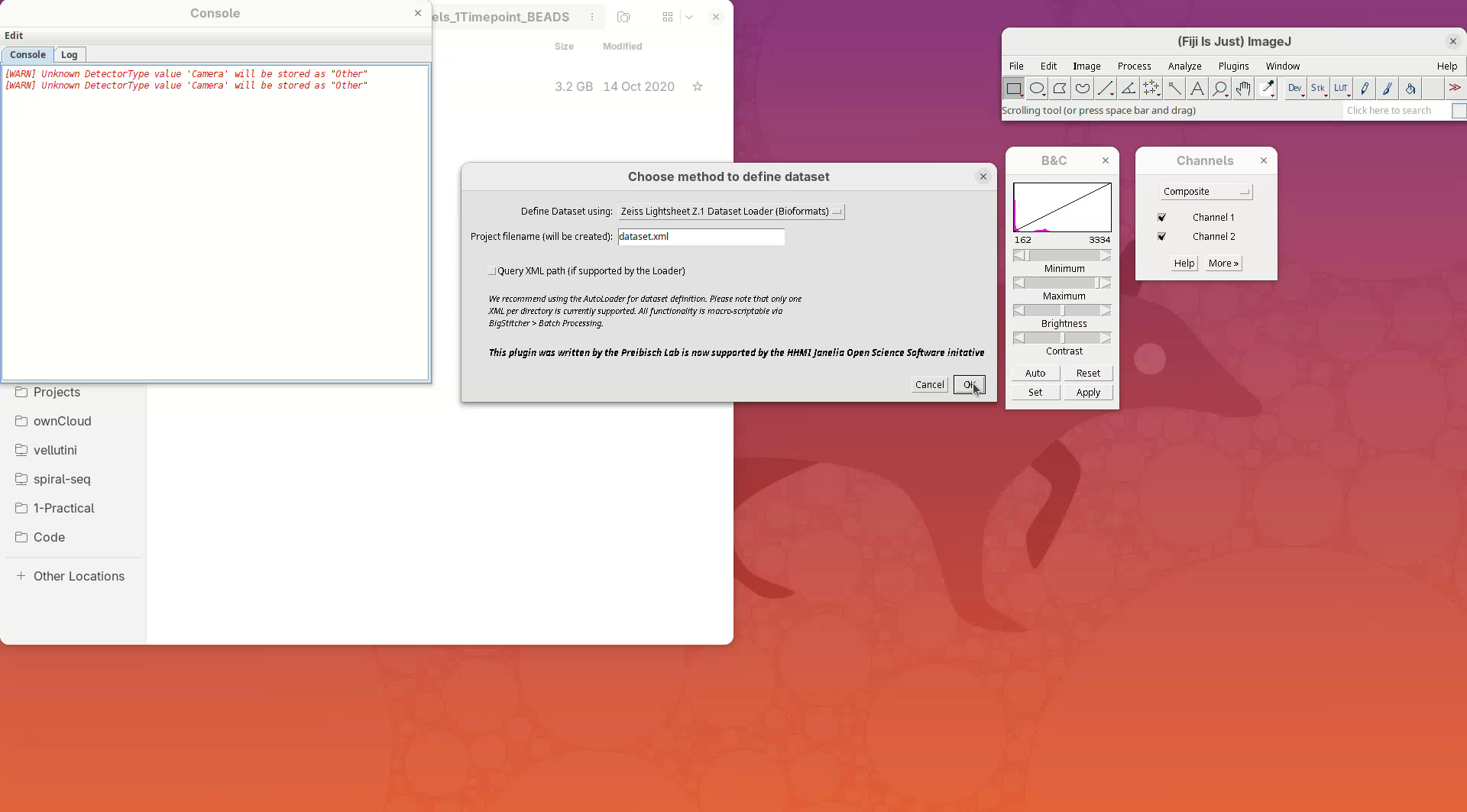
• Click Browse, select the CZI file, and press OK.

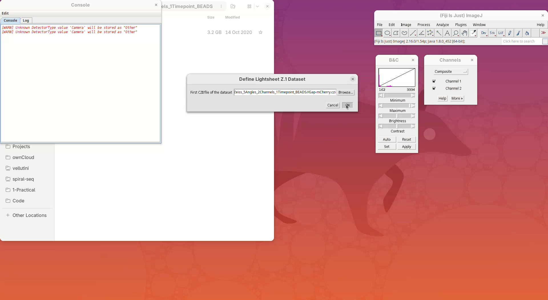
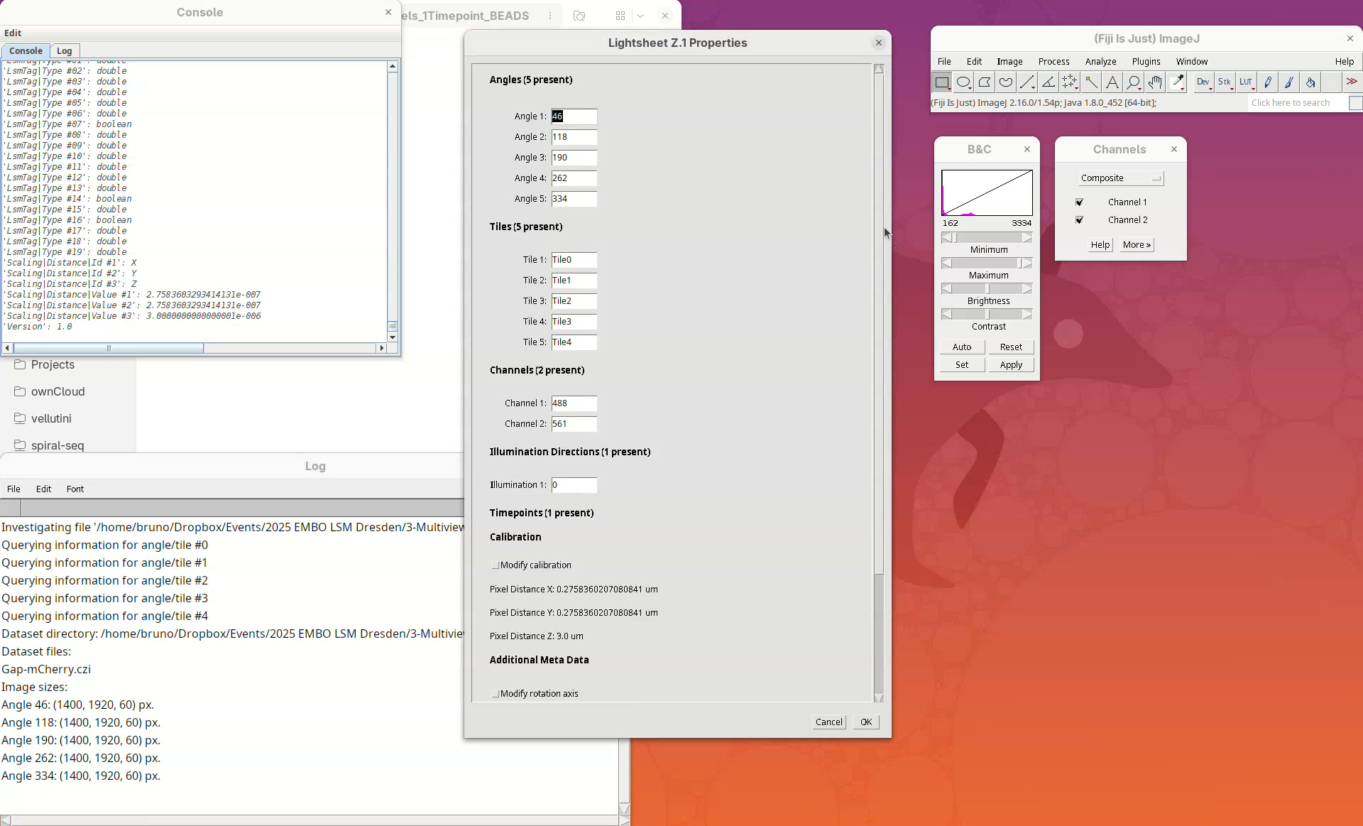
BigStitcher will read the metadata of the CZI and show a dialog with the details.

• Check if five angles are present, if there are two channels, and if the XYZ resolution matches the expected values (see above).
• Then, press OK.

If we look into the working directory, an XML file named dataset will have appeared there.

We can open this file in a text editor to see the information stored there.

• Right-click the file, select Open With... and choose Text Editor.
• The file has the file name, the image dimensions, the XYZ resolution, etc.

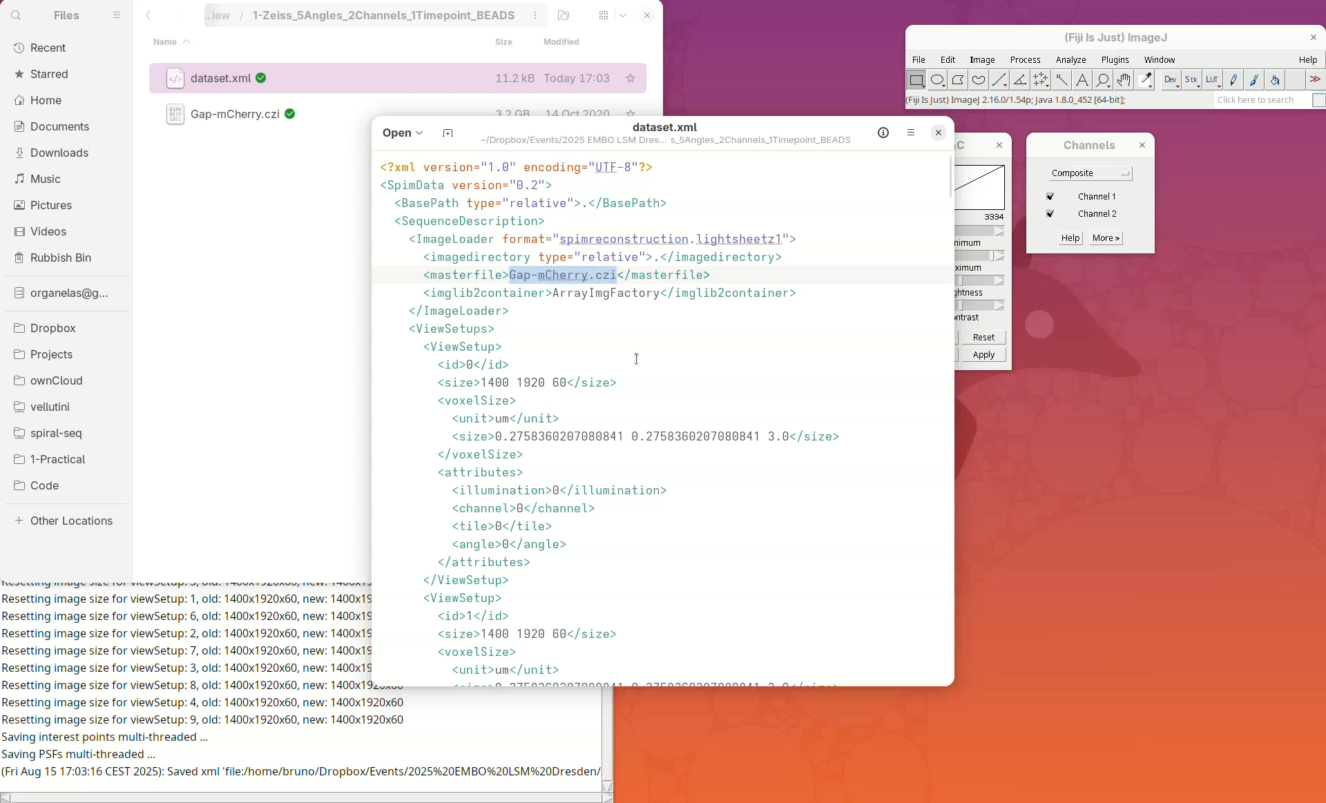
Note: the XML only stores metadata from the dataset and not the actual image data.

Resave dataset

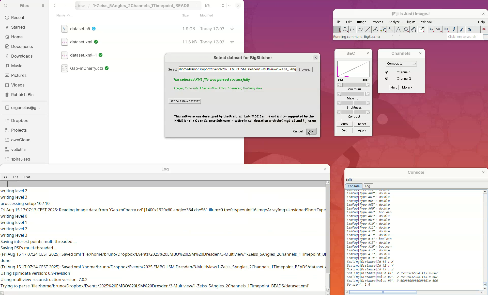
Next, we need to convert the actual image, which is still stored in the CZI, to a format that allows us to open and visualize this heavy dataset in an efficient and lightweight manner. For that, we will resave the data into HDF5 format.

• Go to Plugins > BigStitcher > I/O > Resave as HDF5 (local).

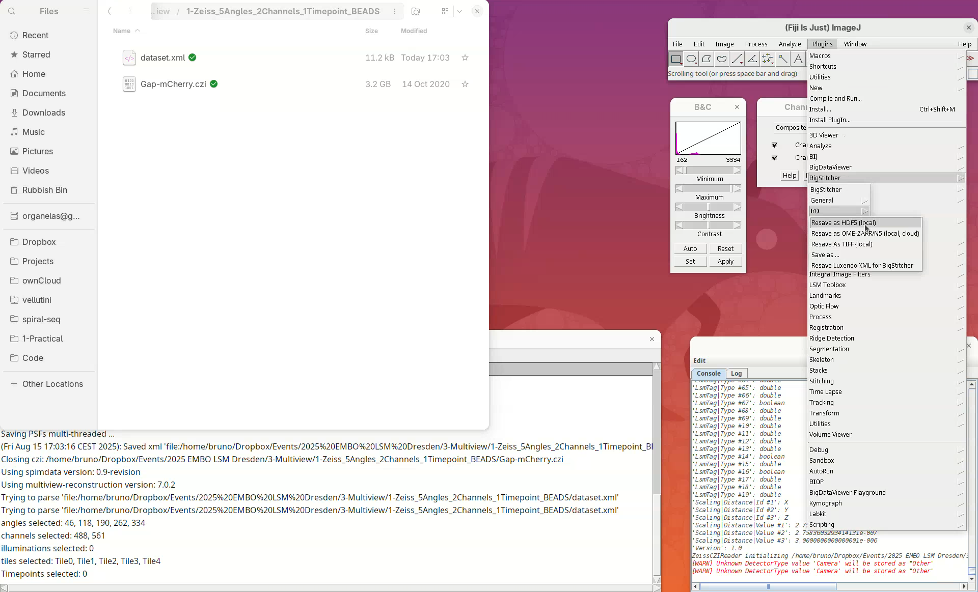
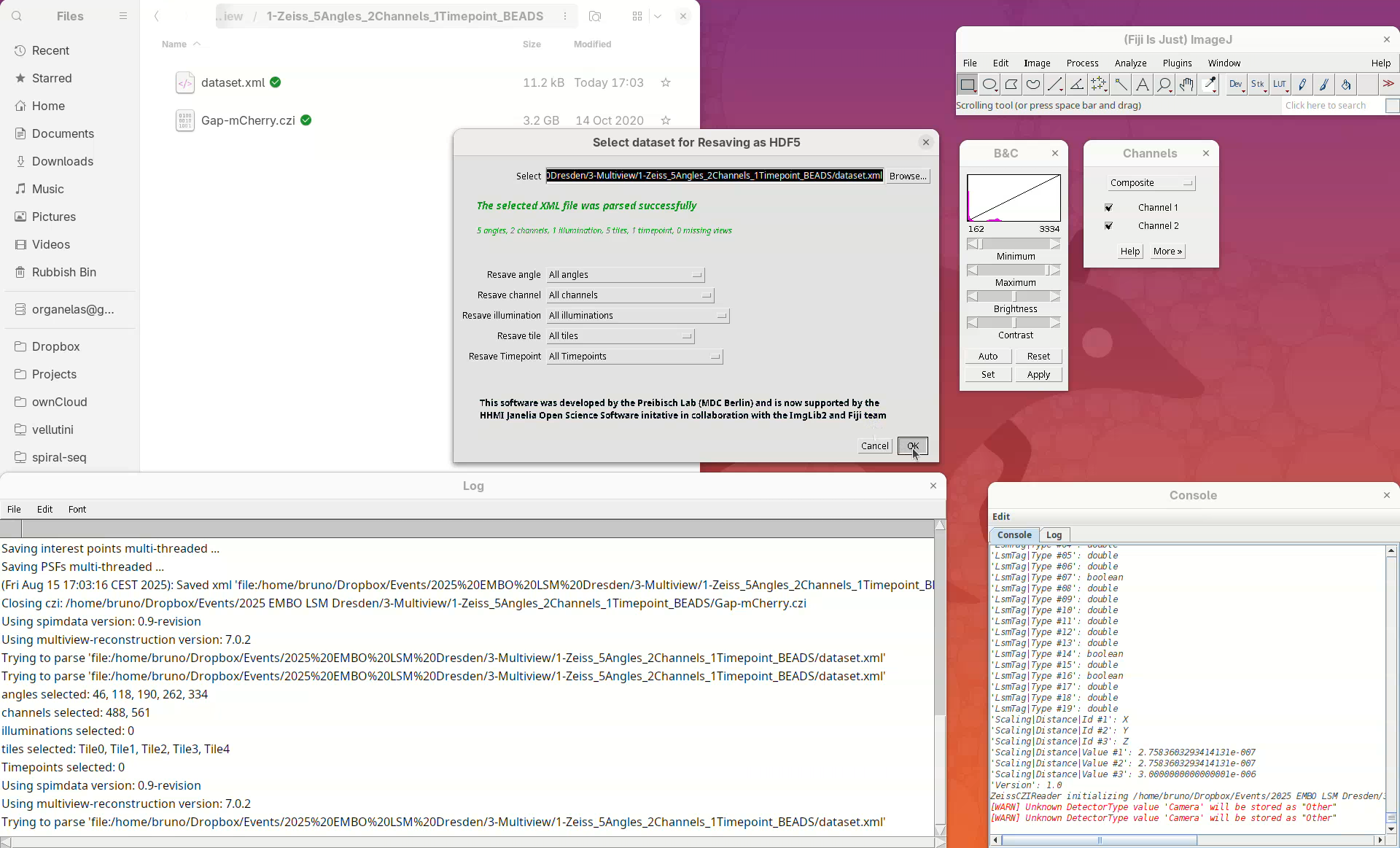
The new window Select dataset for Resaving as HDF5 will automatically load the last used XML file, in this case, our dataset.xml. We can choose whether we want to convert every angle, all channels, all timepoints, or only a subset of those.

• We want it all, press OK.

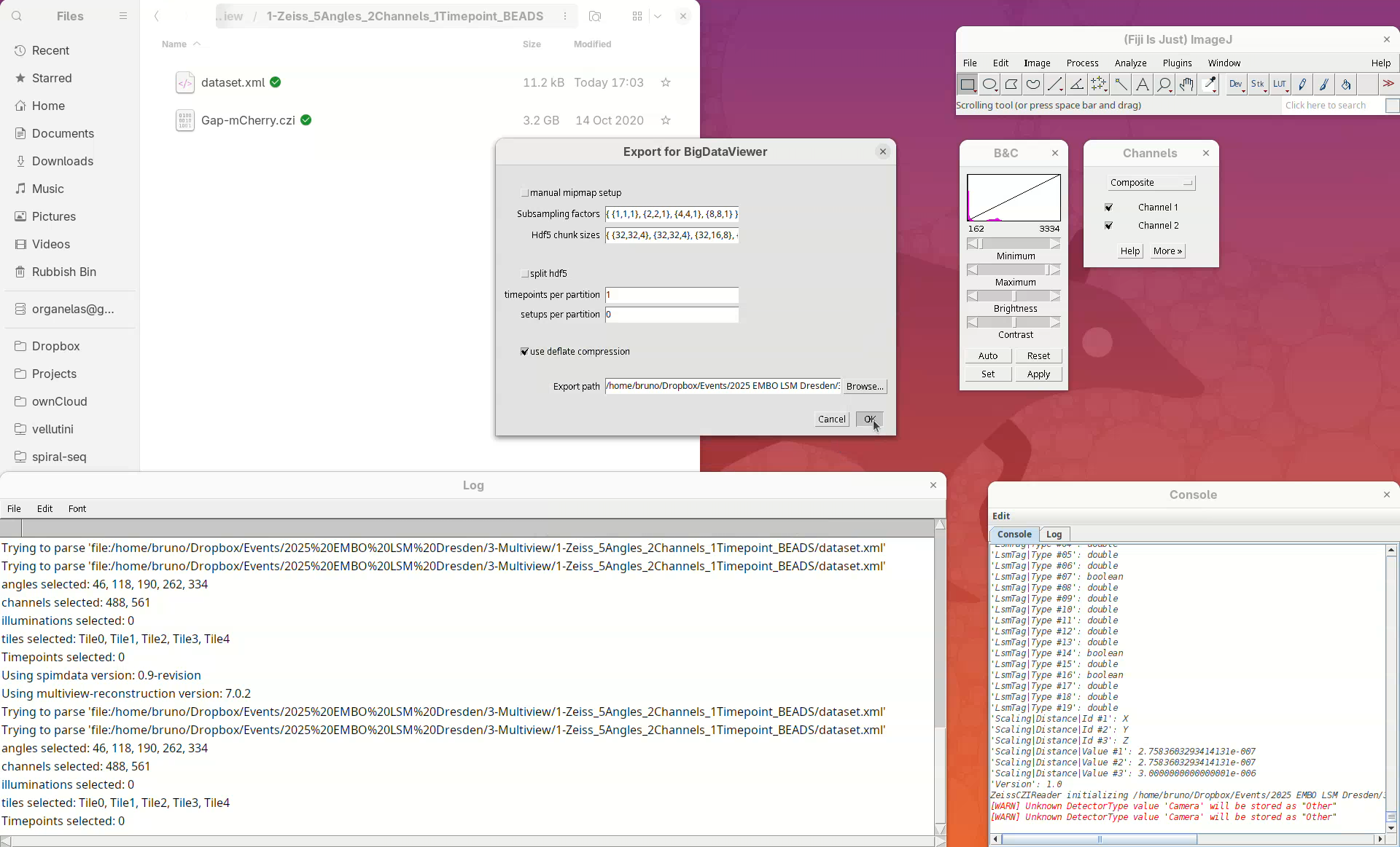
Another window will appear with some resaving options. Leave the options as is, but make sure that the Export path is pointing to the dataset.xml file.

• Click on Browse and, if the file is not selected, navigate and select dataset.xml.
• Press OK and wait…

Resaving this dataset takes about 3 min. However, larger datasets with several timepoints, for example, will take significantly longer. The Log window will show that it’s done.

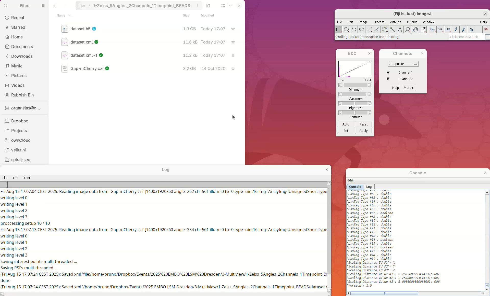
Note that another XML file named dataset.xml~1 and a new HDF5 file named dataset.h5 were created. Every time the dataset file is saved, BigStitcher creates a backup copy. dataset.xml~1 was the original dataset.xml which was renamed after the resaving. If we inspect the new dataset.xml in a Text Editor we will see that it now points to the dataset.h5 file.

• Open the new dataset.xml in a text editor.

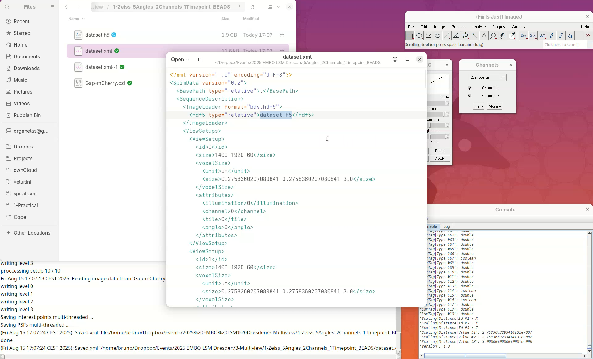
Whenever we refer to the multiview dataset, we mean the XML/HDF5 pair; they are always together.

Visualize dataset

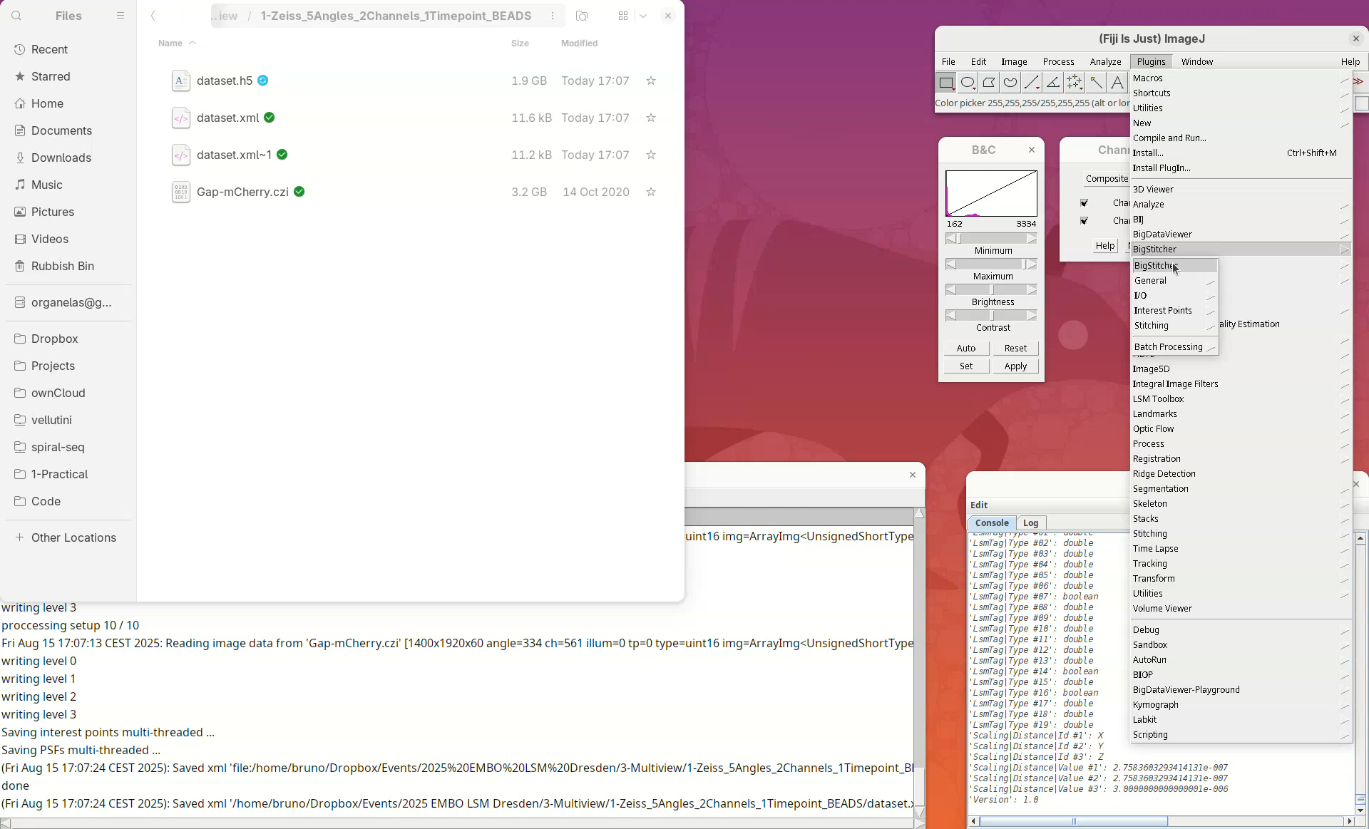
We can finally open the main BigStitcher application and begin the multiview reconstruction.

Start BigStitcher

• Go to Plugins > BigStitcher > BigStitcher.

The last dataset.xml file will be automatically loaded in the select dataset window.

• Click OK.

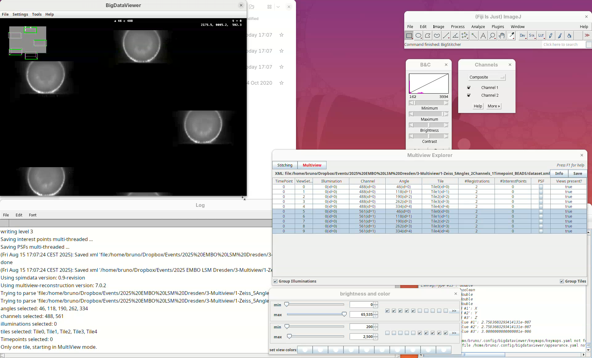
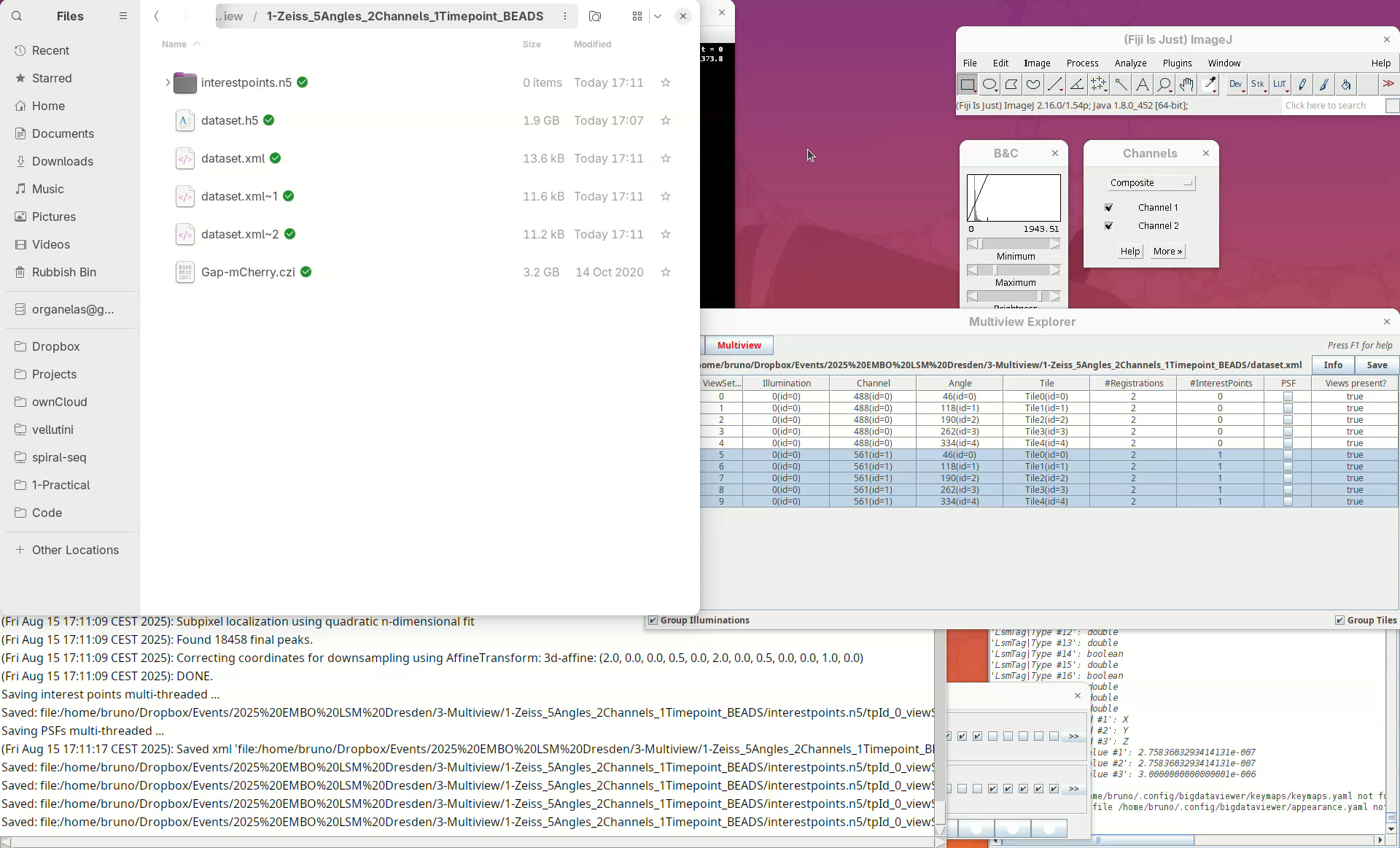
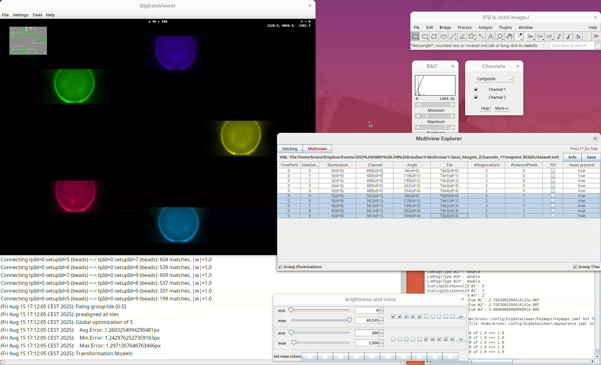
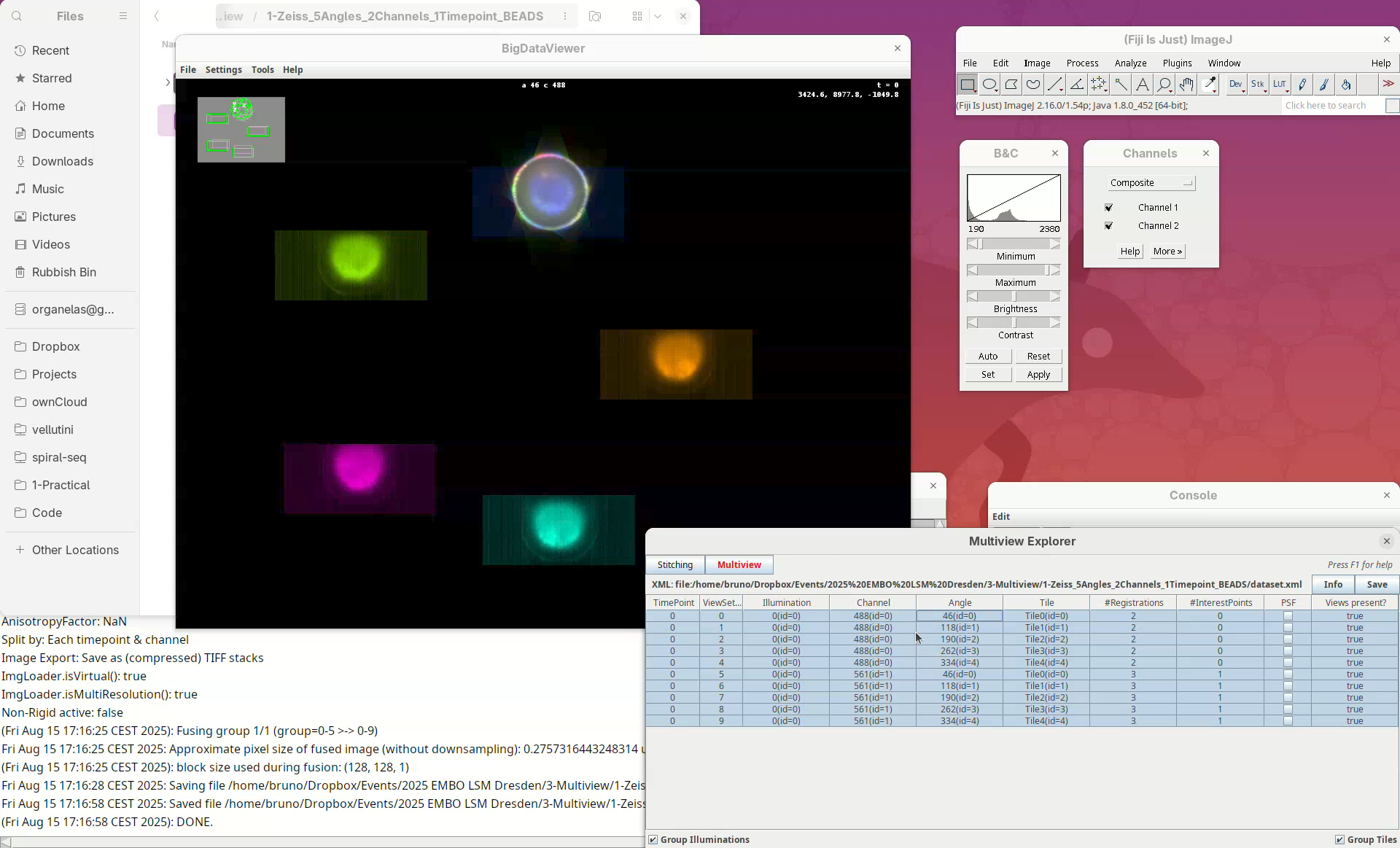
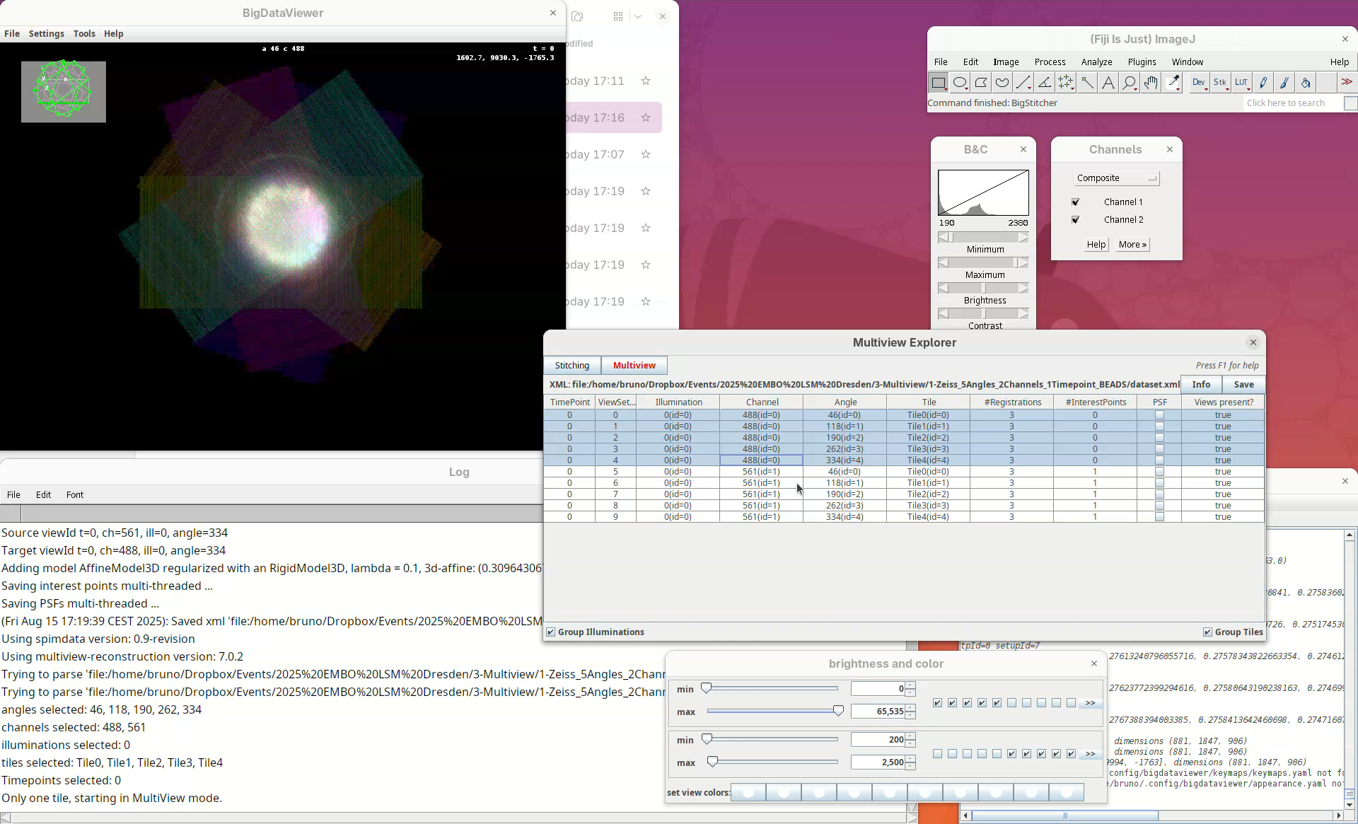
This will open two windows, the BigDataViewer and the Multiview Explorer.

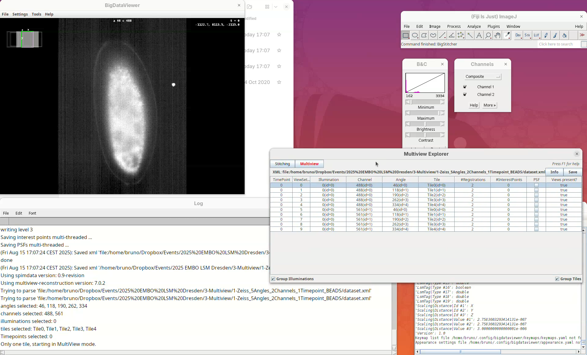
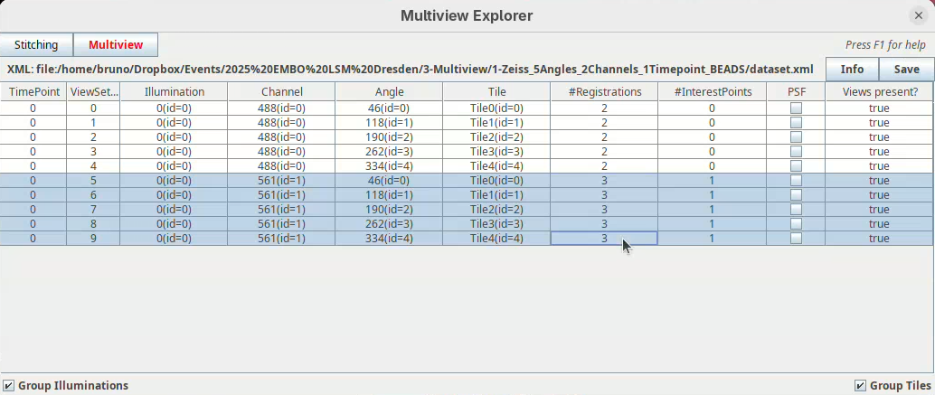
The Multiview Explorer shows a table with the individual views of the dataset. We have 5 views, each with 2 channels. Therefore, we have in total 10 views. Clicking in a row will show the data in the BigDataViewer. We can also sort the table by channel or angle.

• Select multiple rows freely and try sorting it.
• Then, select the five views from Channel 561 (channel 2).

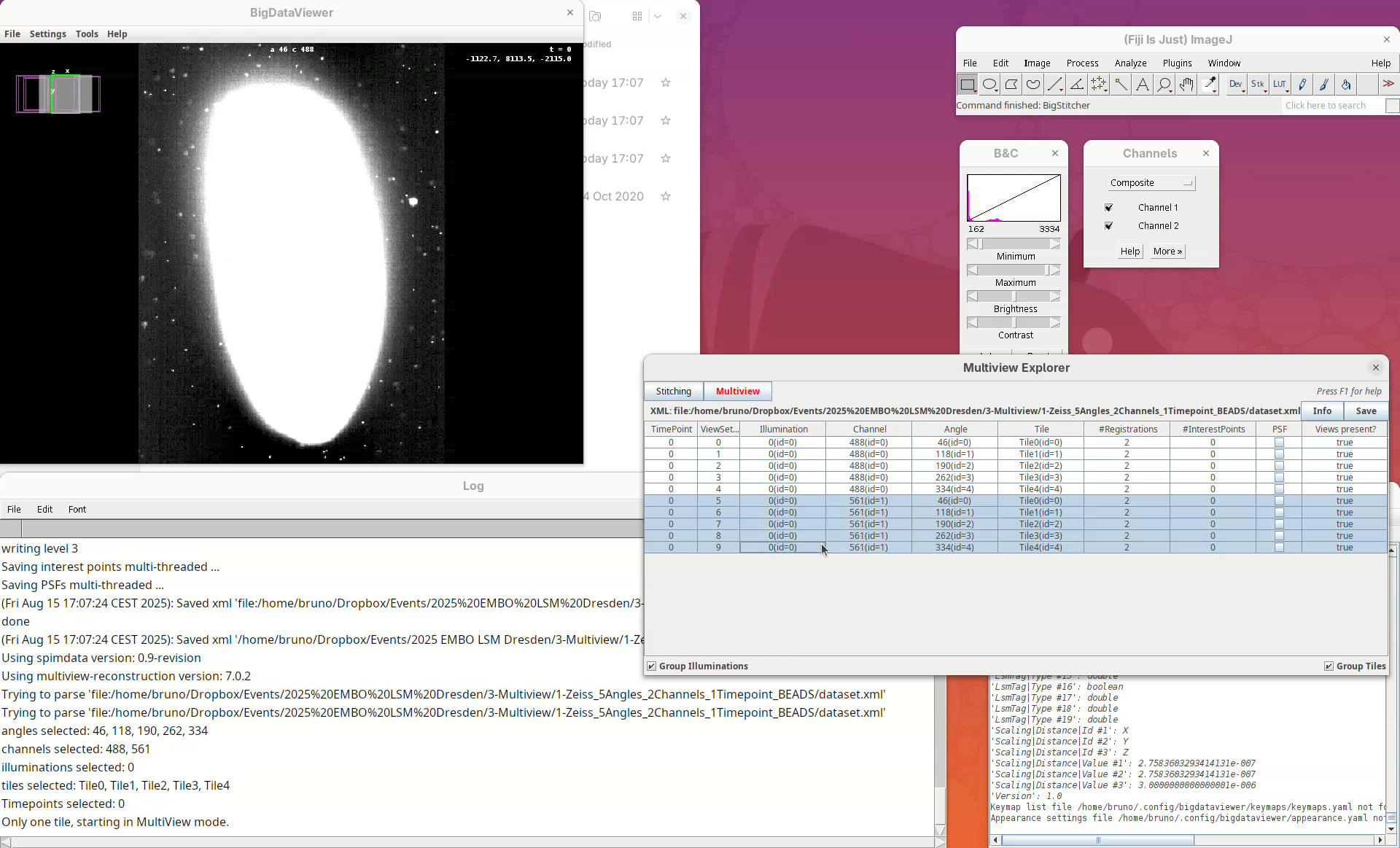
The image is too bright, we need to adjust the contrast.

• Go to Settings > Brightness & Color.

A new window will open.

• Change the max value of channel 2 to 2500.

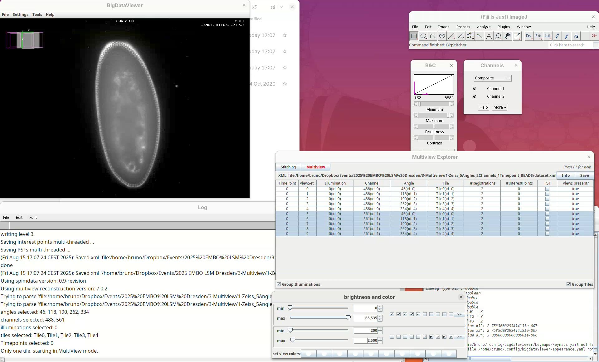
Now we can visualize the dataset in more detail.

Learn BigDataViewer

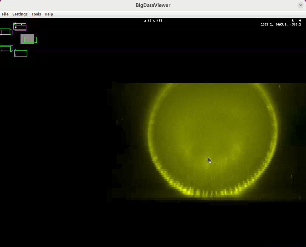
It is important to familiarize yourself with the BigDataViewer commands and shortcuts. BigDataViewer is very intuitive to use but a quick look at the Help is important to not get lost.

Shift+X, Shift+Y, Shift+Z are our compass. If we get lost, pressing one of these shortcuts will get us back to the original XY, YZ, ZX orientation. In this scope the rotation axis is Y. Therefore, pressing Shift+Y will show the different angles from “above”.

• Press Shift+Y and adjust the view to see the five angles.

Some of the most important commands are as follows:

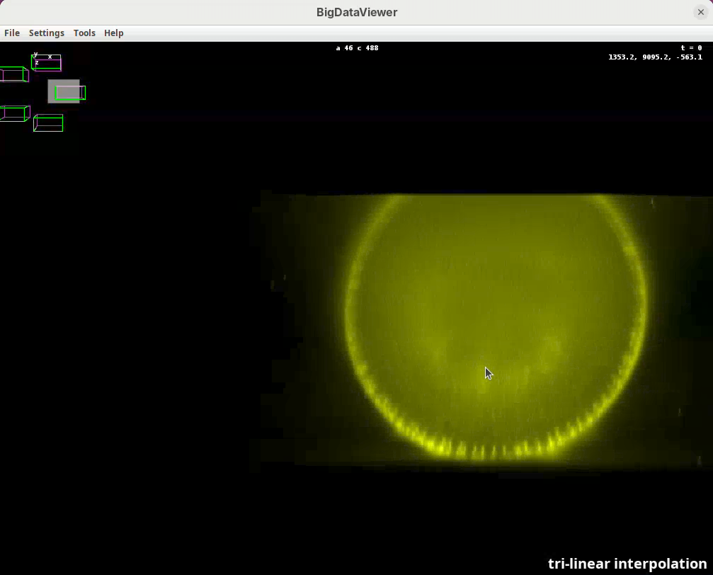
• Left-click and drag to rotate the data around the mouse pointer.
• Right-click and drag to move the view across XY plane.
• Ctrl+Shift+Scroll to zoom in/out fast (Ctrl+Scroll for normal speed).
• Select the BigDataViewer window and press I to activate tri-linear interpolation for better visualization.

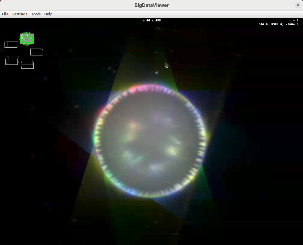
• Select the Multiview Explorer window with the five views selected and press C. This will autocolor the views which is great for visualization.

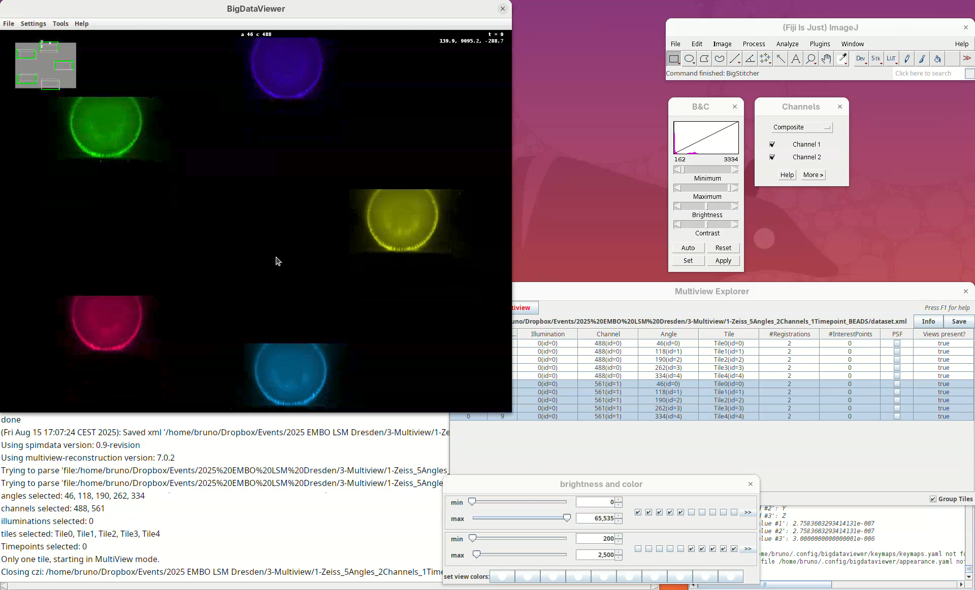
Take some time to explore the data, the different views, zoom in and out, find the beads, and get familiar with the BigDataViewer. Then finish with the 5-views oriented as in the image above.

Detect points

We can now start the first processing step of the pipeline, detecting points of interest to be used for the registration. The Multiview Explorer is always the starting point.

• Select the five views of channel 561 (if not selected).

In this case, we want only the views of channel 2 to be selected since it is in this channel that the beads are visible.

• Then, right-click the rows with the mouse.

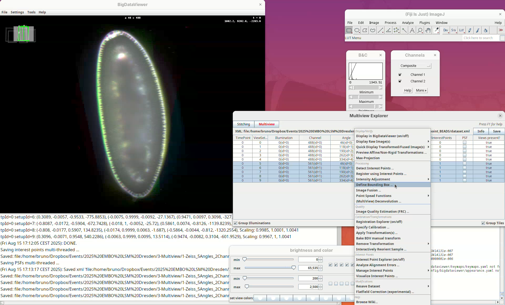
A long menu will appear. This is the main menu of BigStitcher. Anything that we select will only be applied to the selected views.

• Find the section Processing and select Detect Interest Points....

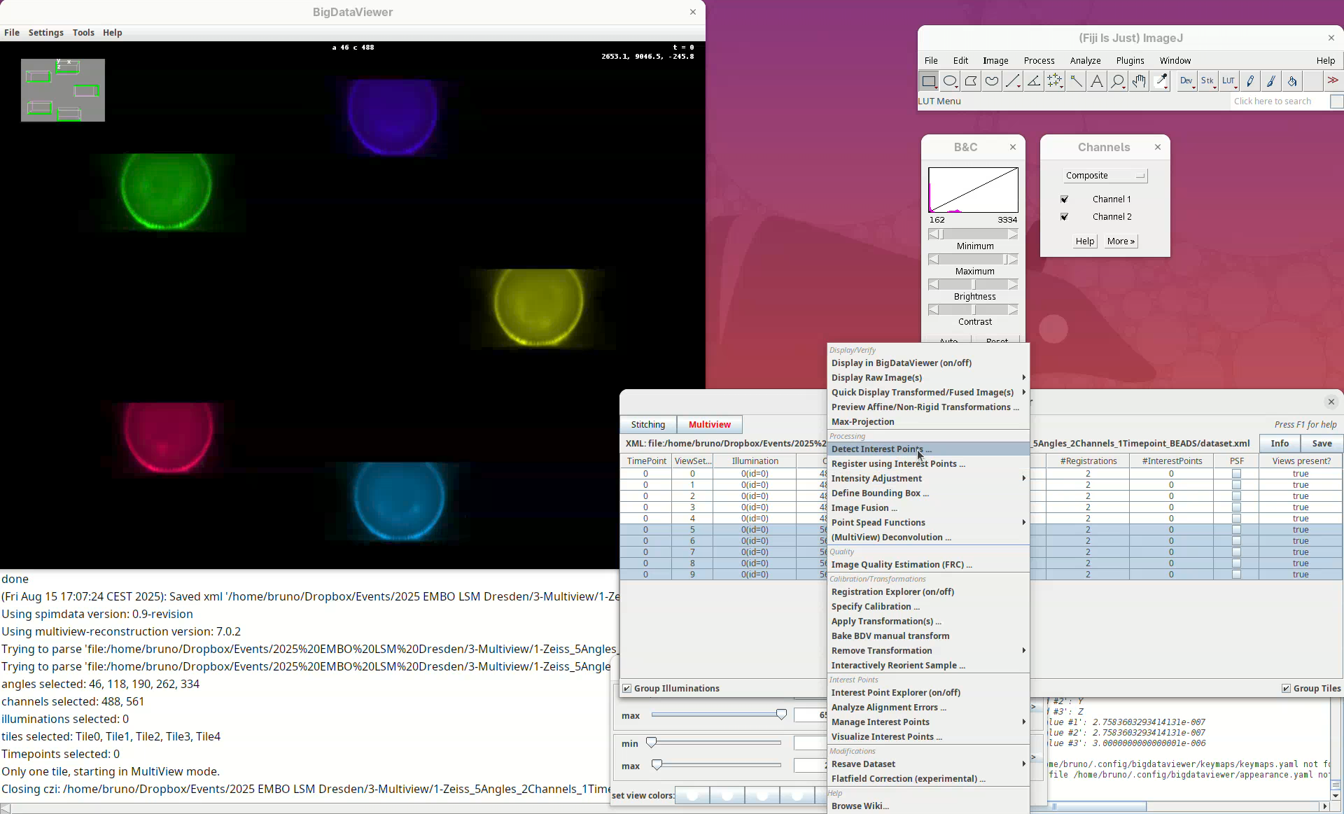
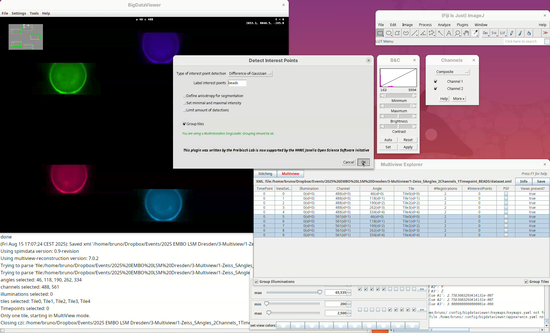
In this first window we can choose the Type of interest point detection (Default: Difference of Gaussian) and a label to describe these interest points. One dataset can have multiple sets of interest points.

• We will keep the default options and press OK.

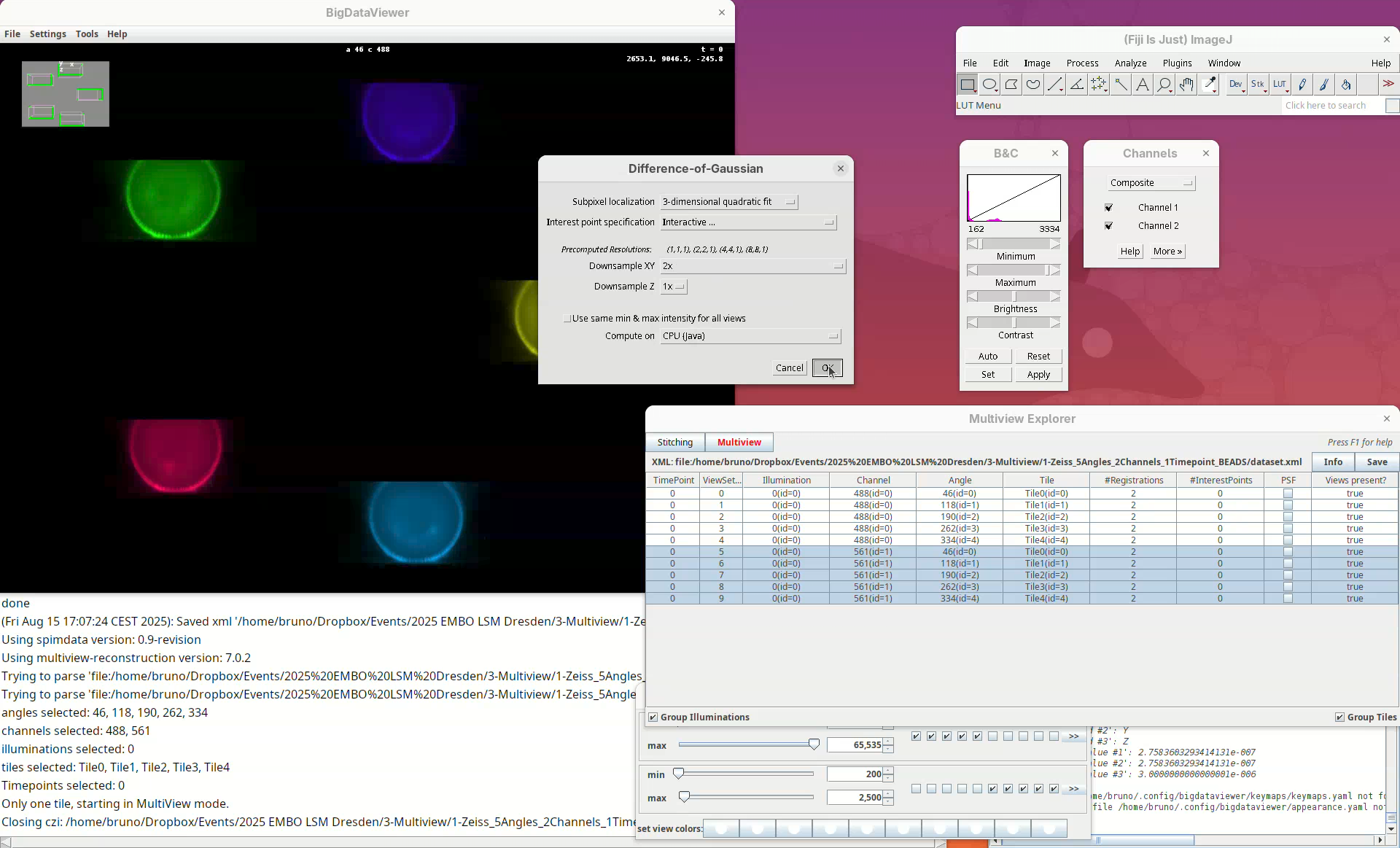
We can set different parameters for the Difference of Gaussian approach. What is important to us at this point is to make sure that Interactive... is set for Interest point specification and that we change Downsample XY from Match Z Resolution (less downsampling) to 2x. The latter is not essential for all datasets but it works better for this dataset which has relatively high anisotropy (lower Z resolution compared to XY). Keep Downsample Z as 1x.

• Press OK.

In this case, we can select which view we will open the interactive window for and if we will load the entire stack.

• Press OK to load the entire first view.

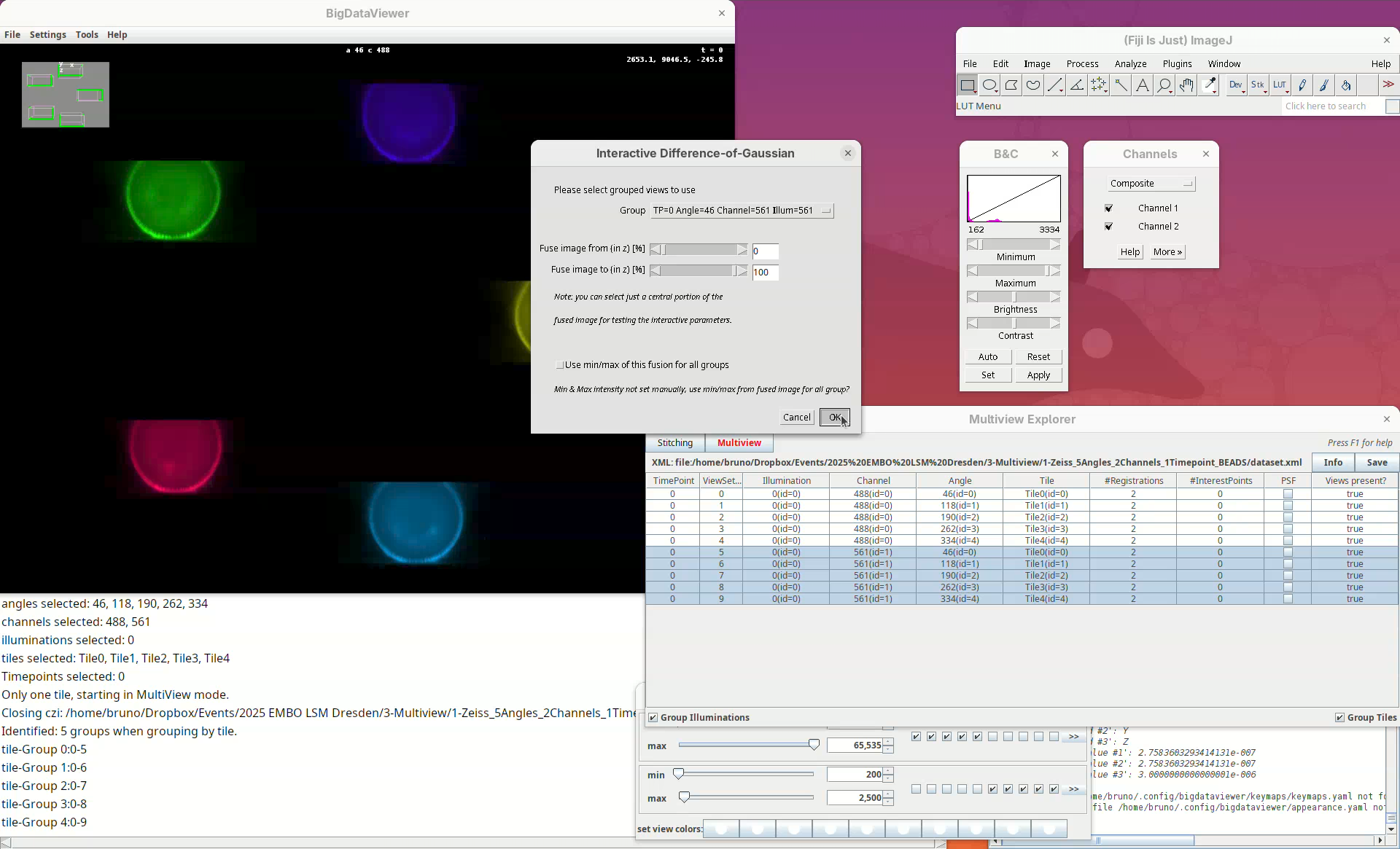
A stack will open with a rectangular ROI placed at the top left corner. The ROI shows a live view of detected points for the current parameters Sigma and Threshold in the other window.

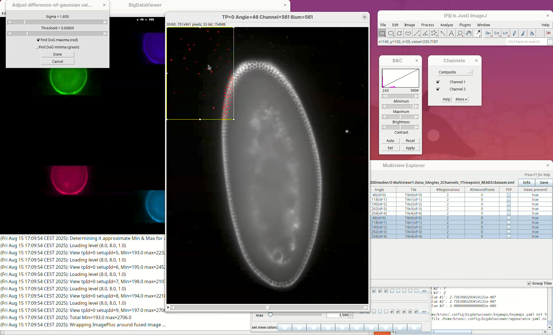
Sigma is the size (radius) of the point and Threshold is the intensity-based cut value to discard low-quality detections. The default is to Find DoG maxima (red), in other words, bright spots. We can also find dark spots surrounded by bright areas (useful for some samples). Note that this is a normal ImageJ window, so we can zoom, adjust contrast, and if we lose the ROI, we can simply draw a new rectangular ROI. We can drag the ROI around by clicking inside it and holding and dragging it.

What we want to do now is to adjust the Sigma and Threshold so that most of the beads outside the embryo are properly detected with the least spurious detections. The best way to begin is to:

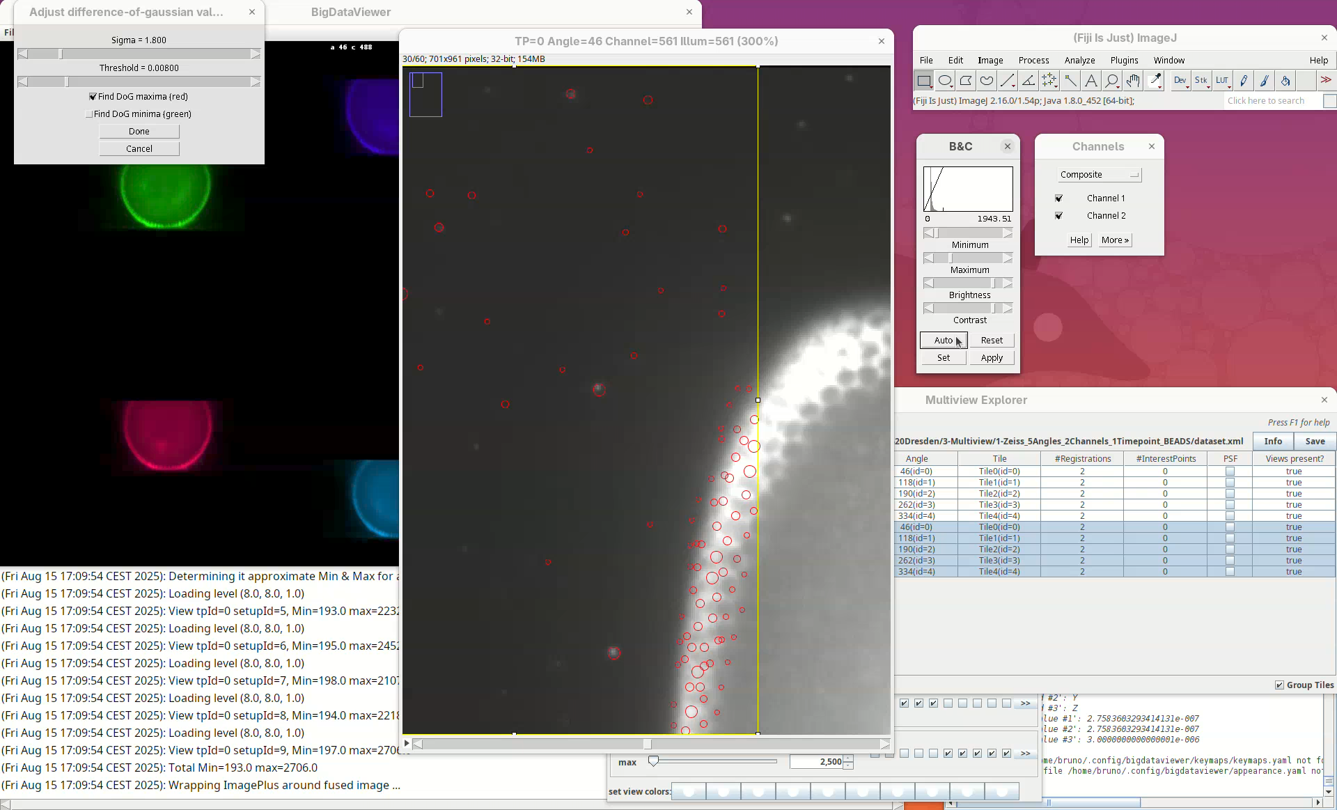
• Zoom in on a bead outside the embryo.
• Check if the circle size is matching well the bead.
• Move the Sigma slider, aiming for a circle slightly larger than the bead.

Remember to also move through the Z slices of the stack to see how the detection behaves.

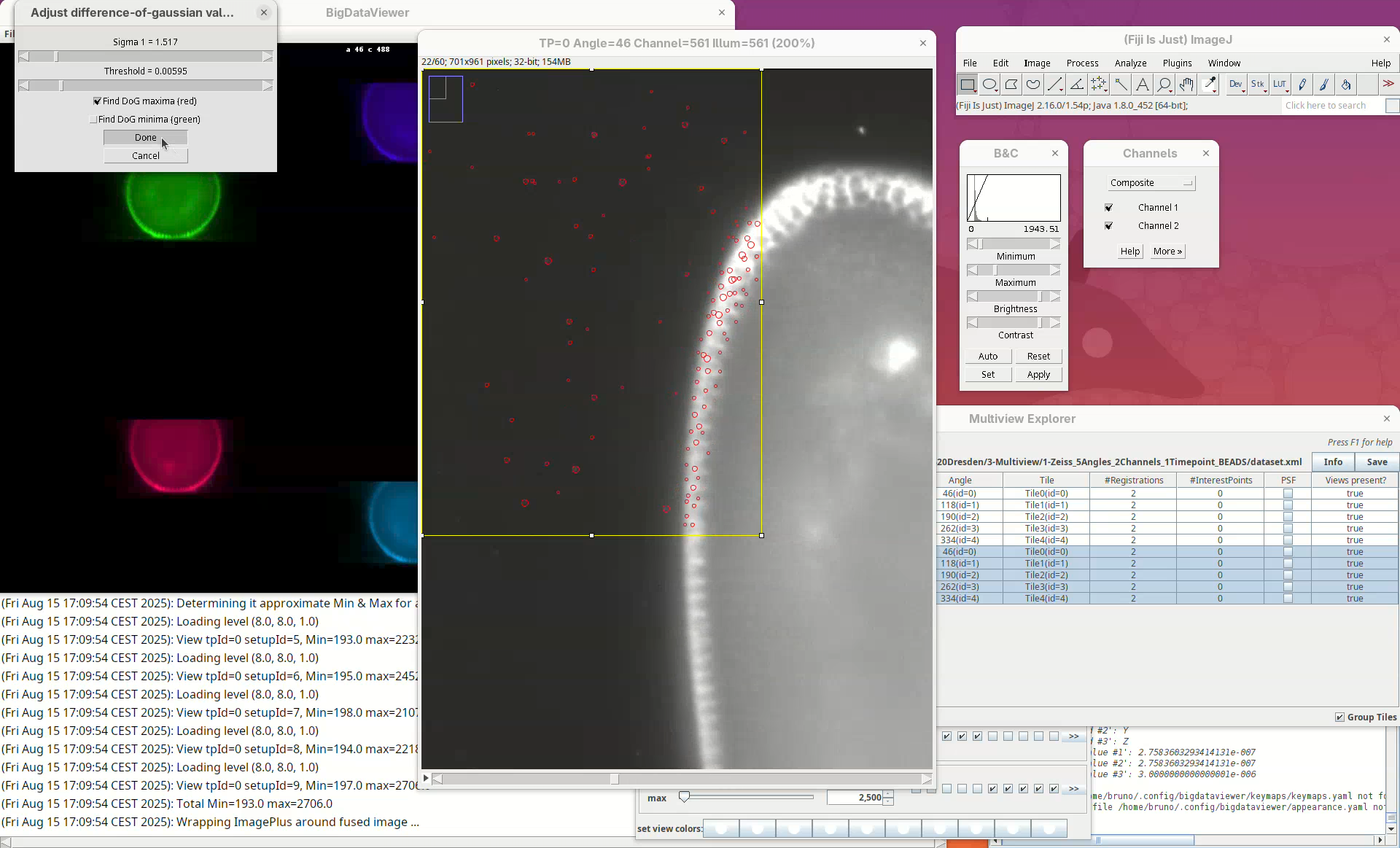
• If the size looks good, increase the Threshold until real beads begin to not be detected, then roll the slider back until most real beads are detected.

Note that, no matter how much we tweak these parameters, there’ll always be many non-bead detections in the sample tissues. These detections will not have a strong influence on the registration given that we have enough real beads in the sample.

• When satisfied, press Done.

Bead detection takes some time.

• Once DONE, go to the Multiview Explorer window and press Save.

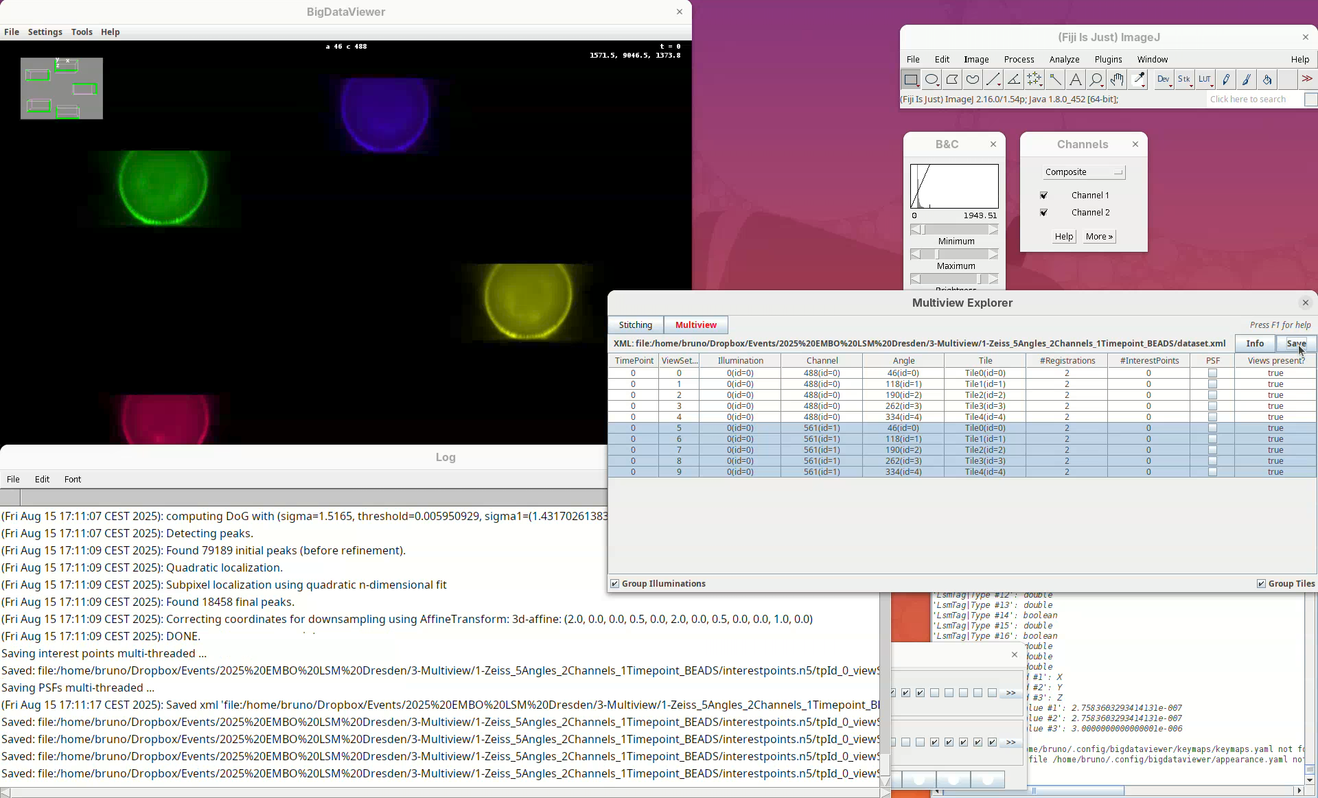
This is important because the detections are initially saved in memory and will only be written to disk after pressing Save (detections are saved in a directory named interestpoints.n5).

Note that the column #InterestPoints in the Multiview Explorer now shows 1 for the five views of channel 561 (but not for channel 488).

Register views

Now we can try to register these views using the detected interest points.

• With the 5 views selected, right-click and run Register using Interest Points....

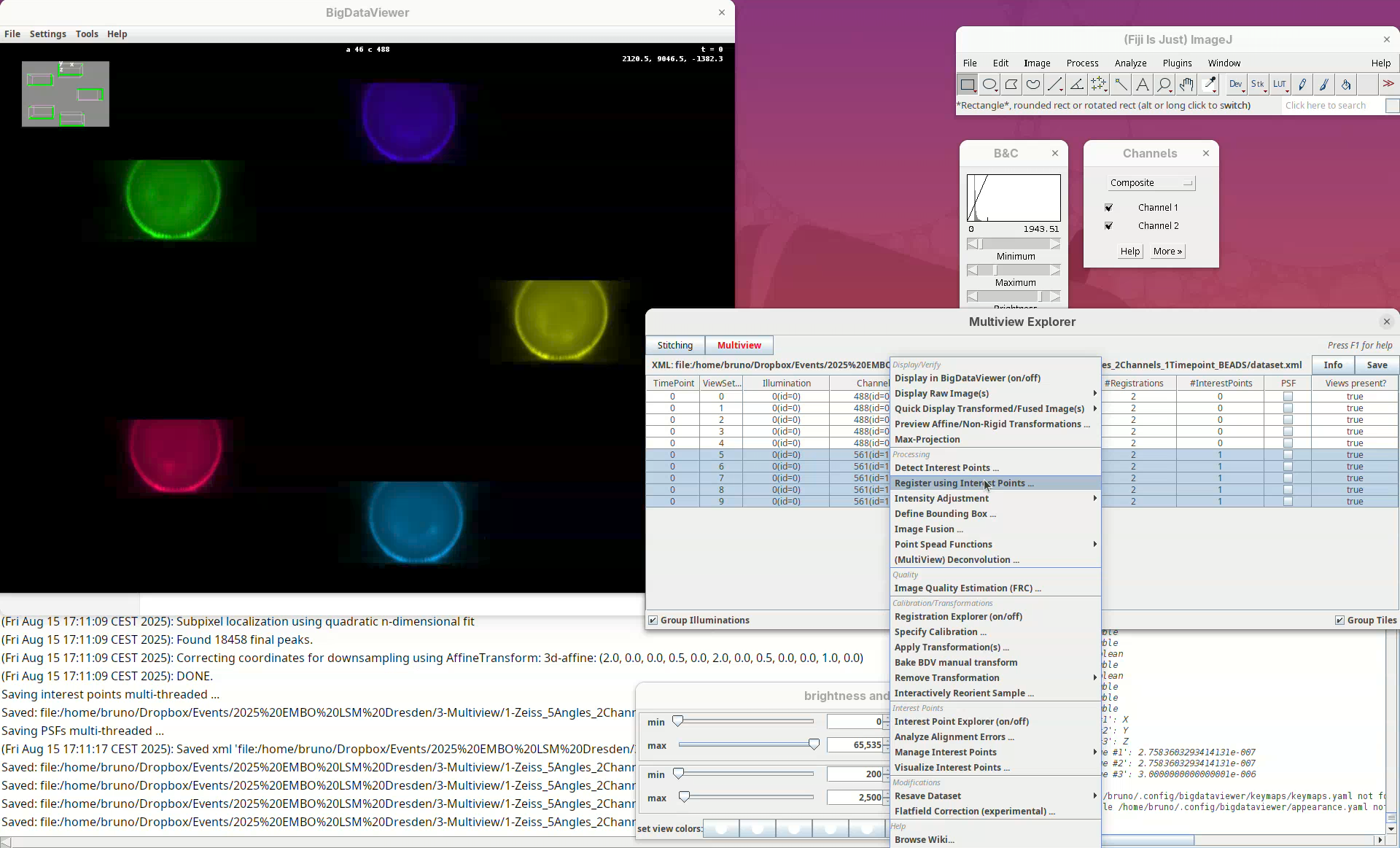
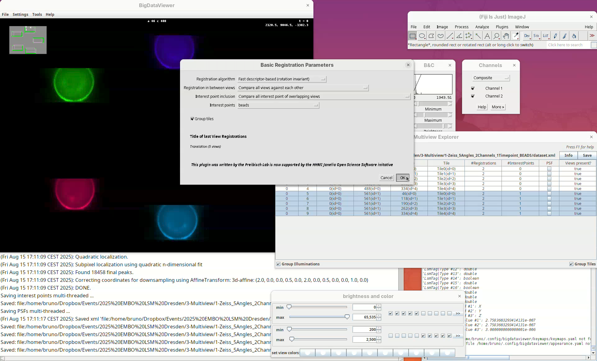
We can change different registration parameters like the algorithm to be used or the specific set of previously detected interest points. We want to go with the default Fast descriptor-based (rotation invariant) as Registration algorithm since this works well for bead-based registration with Z.1 datasets.

• Because our views have almost no overlap, change the option Registration in between views to Compare all views against each other.

Leave the other options as is making sure we are using the Interest points labeled as beads.

• Press OK.

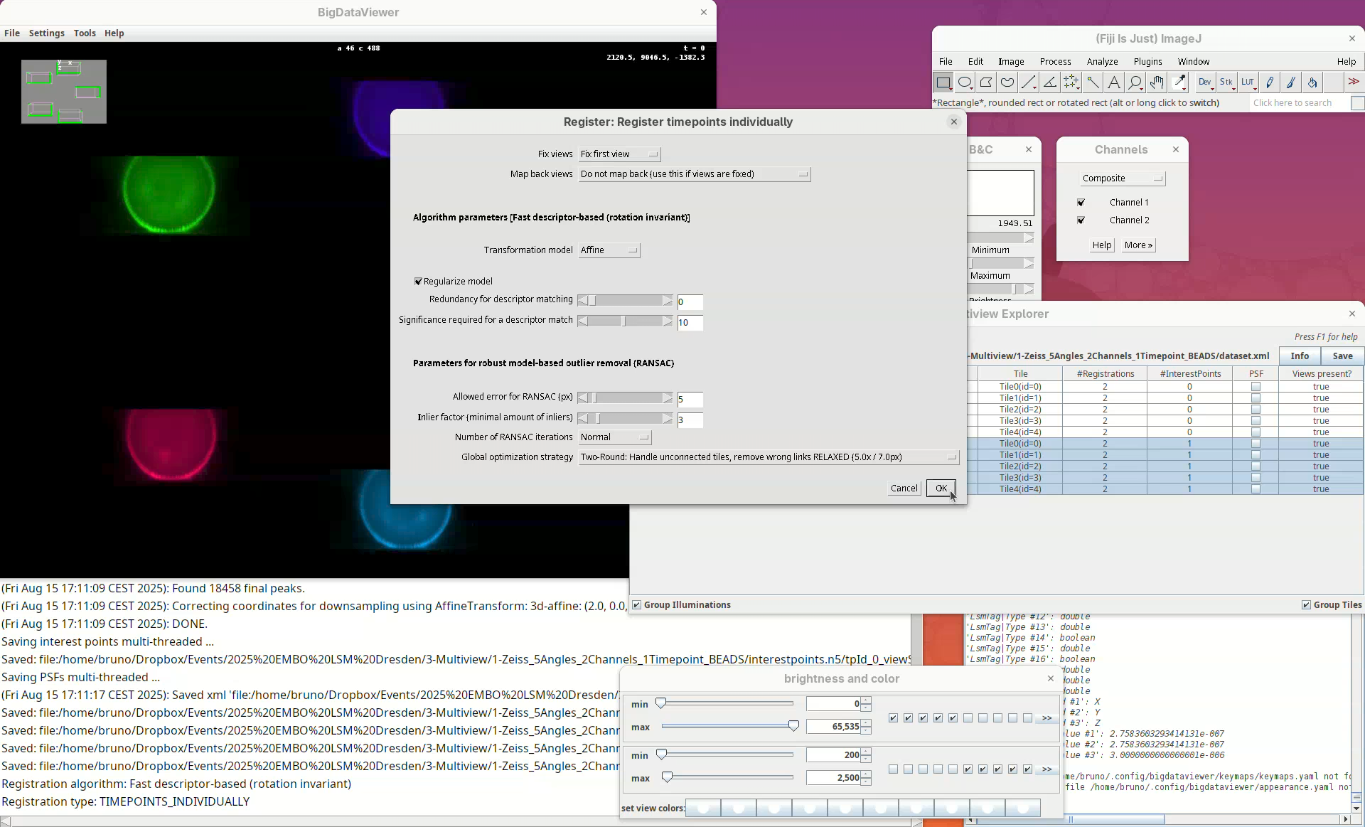
A window will open with several other parameters to tweak. Please refer to the BigStitcher documentation for the specific function of these. For us, it is important to note two.

The option Fix views set to Fix first view means that all other views will be mapped to the first angle. The option Transformation model set to Affine means that the data will be transformed non-rigidly to fit the individual views. This is important since different portions of the stack might have a certain degree of distortion from the objective lenses and an affine transformation helps to fit the views better together. The other parameters we will only need to change if our initial registration fails.

• Press OK.

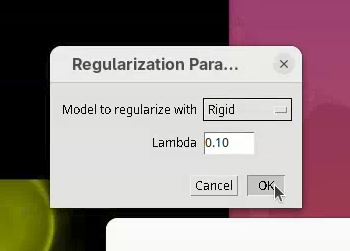
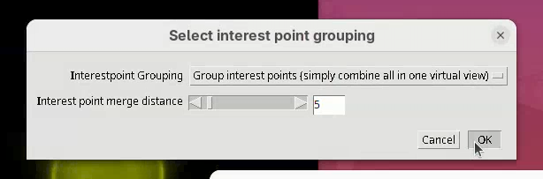
The next two small windows to open, Regularization Parameters (Rigid and 0.10) and Select interest point grouping (Group interest points and 5) can be kept as is.

• Press OK on both.

The registration will begin and be over in a few seconds. Don’t blink or you will miss it! If successful, you will see that the individual views will now have moved over (registered) the first view and they are all overlapping in the BigDataViewer window.

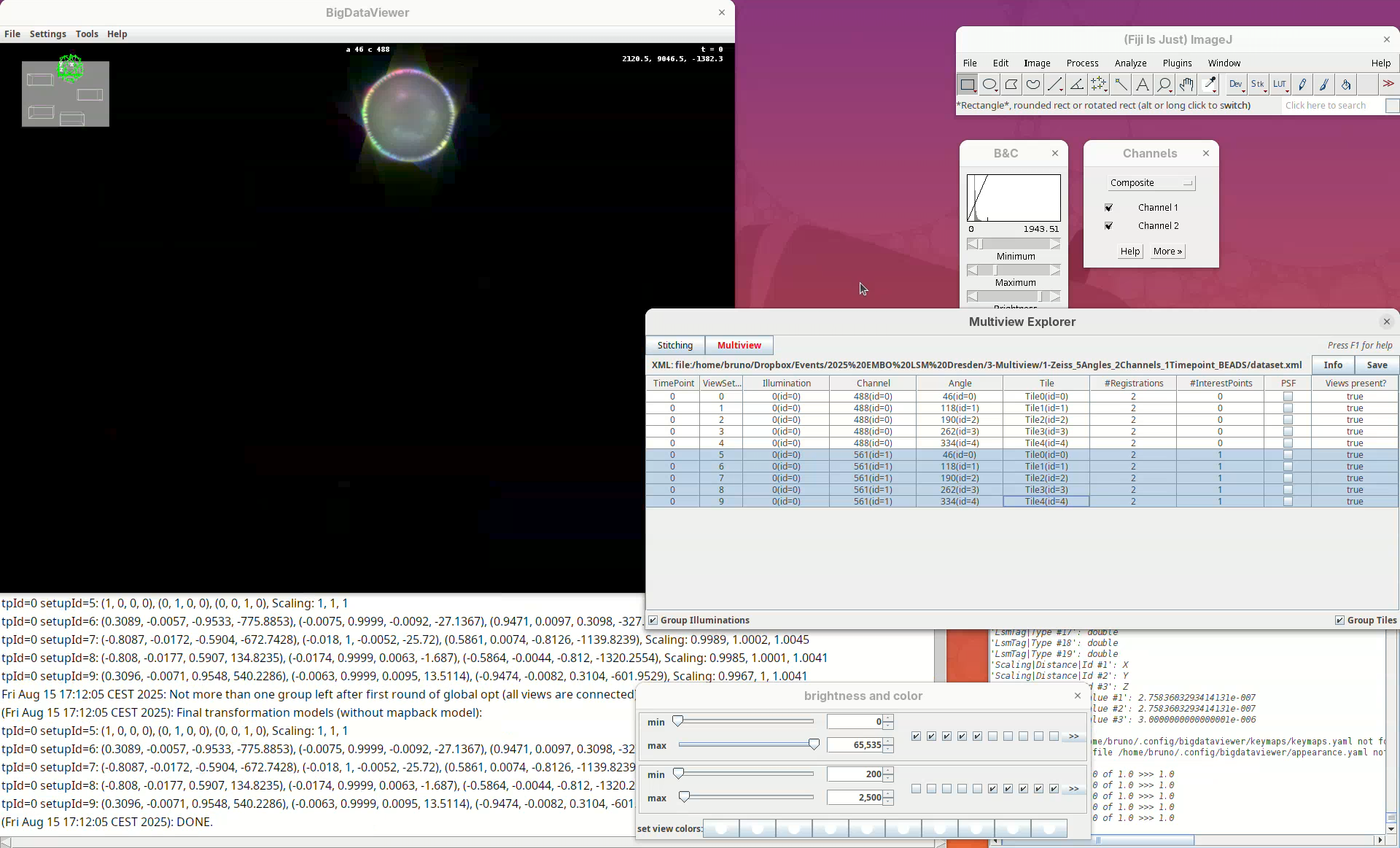
Now that the views are registered, explore the dataset to verify that the registration worked well. The best way to do this is visually. One of the first things that you can do is to:

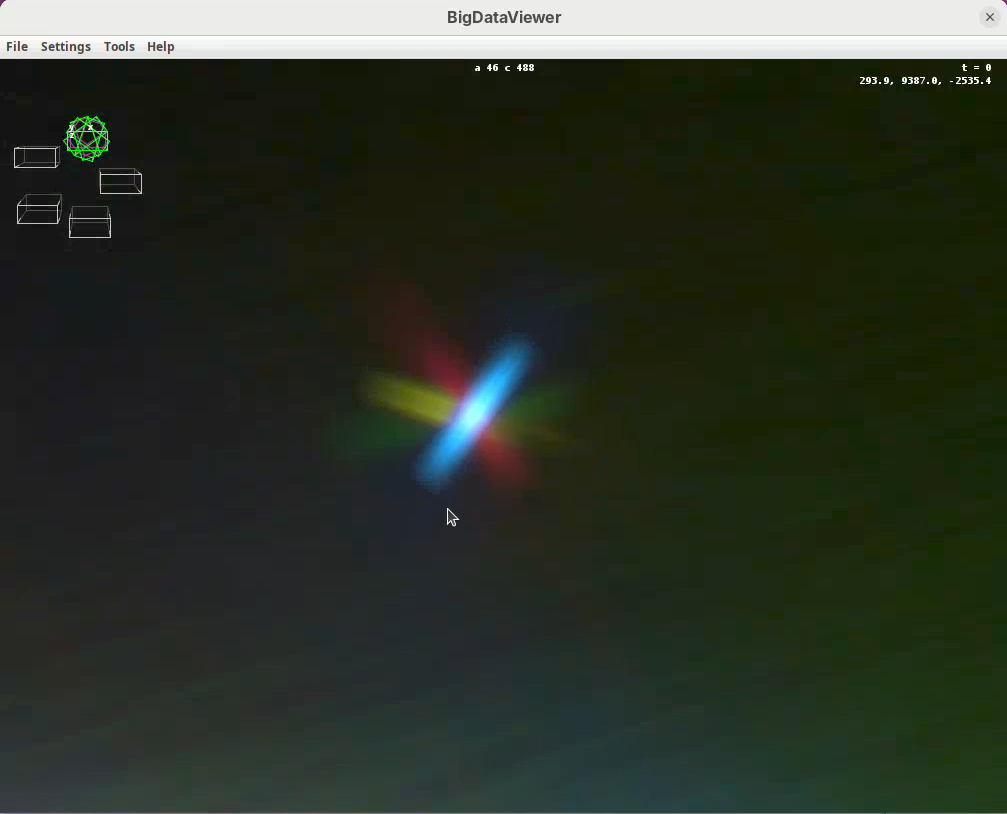
• Press Shift+Y and zoom in on a bead close to the embryo’s surface.

You will see the point spread function of one bead in each individual view forming a star with generally four views (as the fifth view is too far away). If the sample is registered well, the center of the point spread functions of the different views should match in the middle of the star.

Another thing that you can do is to find a structure you know well in the sample and check that the tissues are actually registered. It can happen that the beads are nicely registered, but the tissues themselves are a bit off.

• When done checking, make sure to Save the project again.

After saving, the #Registrations column should now show the number 3 for the selected views (if not, deselect and select them again to update the counter).

Set bounding box

Our dataset is now registered, but before fusing the views it is important to set a bounding box around the sample. This reduces the final dimensions and file size of the fused data.

• For that, right-click and select Define Bounding Box....

We want to define it interactively, so leave the Bounding Box option as Define using the BigDataViewer interactively. You can give the bounding box a custom name and define different bounding boxes for different purposes, but the default name is good enough for this tutorial.

• Click OK.

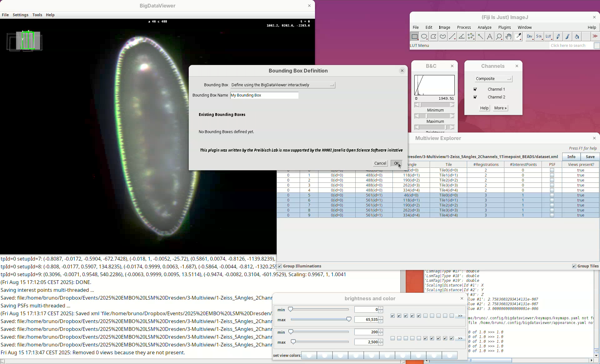
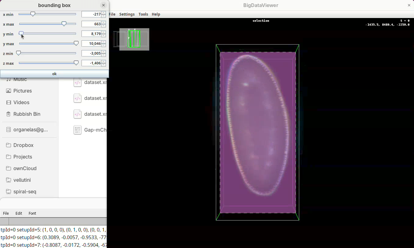
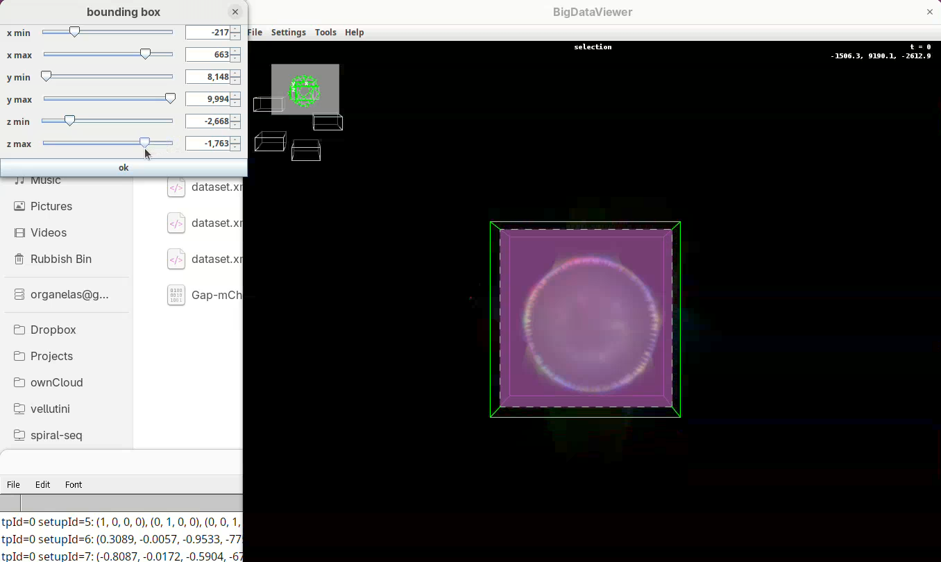
Two windows will open: BigDataViewer with the sample and some purple shade and a bounding box window full of sliders.

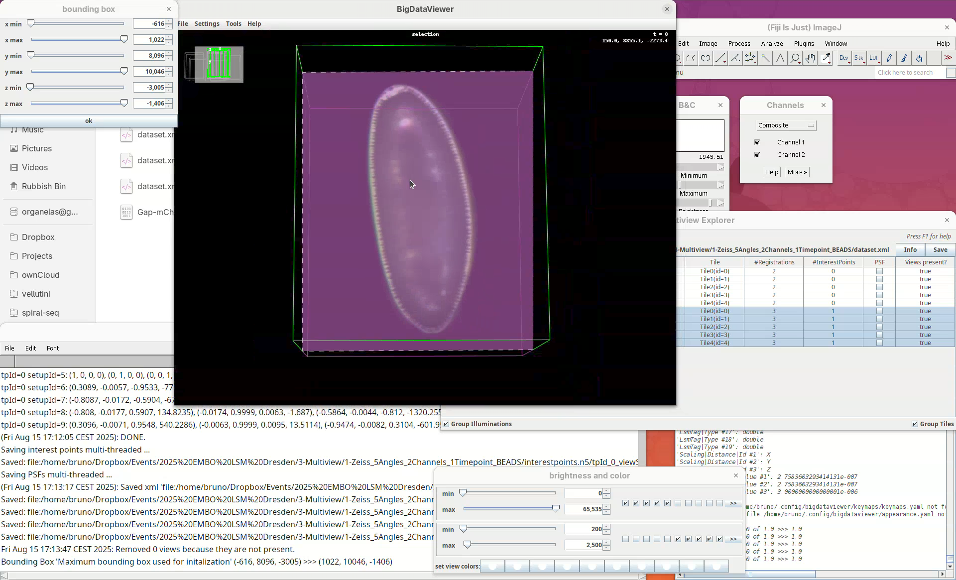
For defining the bounding box I follow a specific procedure, always in the same order, to avoid inadvertently leaving out a part of your sample when fusing.

• First, press Shift+X to orient the sample on XY.

• Go through the sample (Z) top to bottom to get a sense of the entire volume and stop back at the middle.

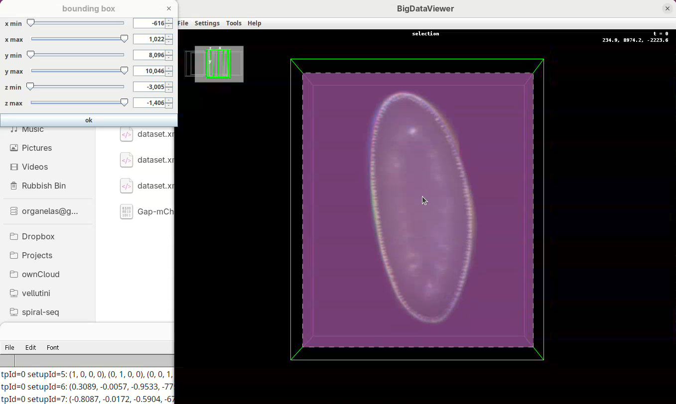
• Move the x min slider to the right to cut out the region on the left of the sample (the dashed line is the reference edge).
• Get close to the sample, but leave a gap.

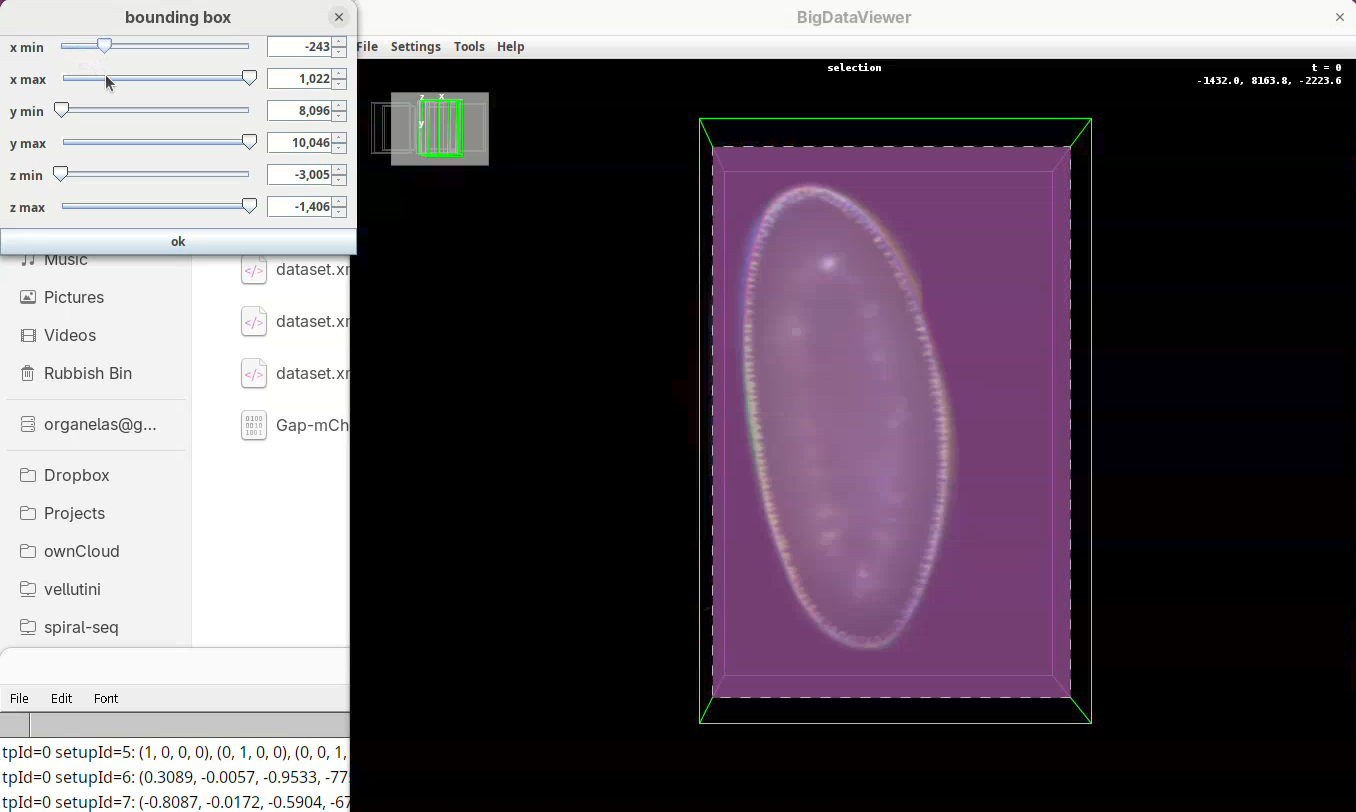
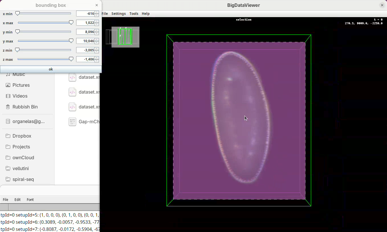
• Once the x min is set, go again top to bottom through Z to make sure nothing was cut out.
• Now do the same for x max to cut out the region on the right side of the sample.

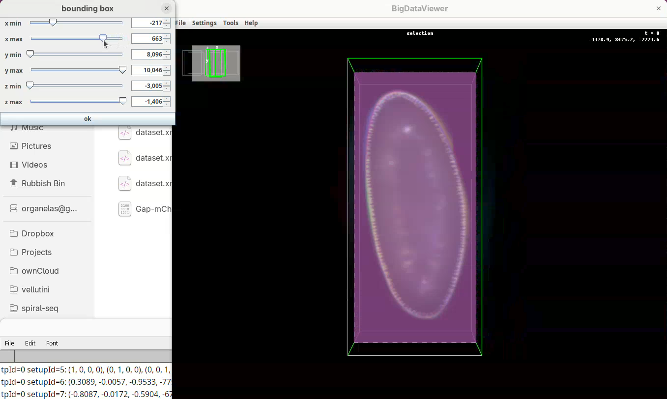
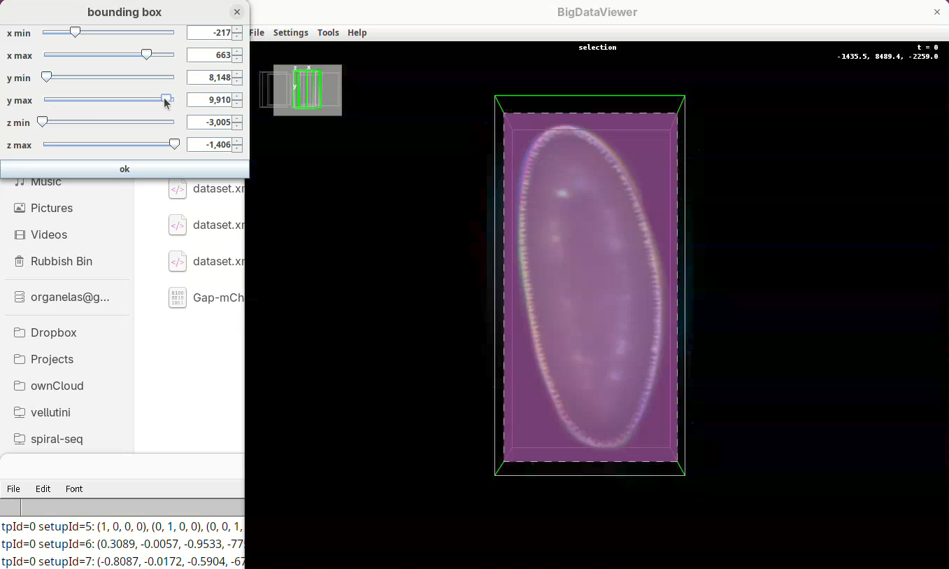
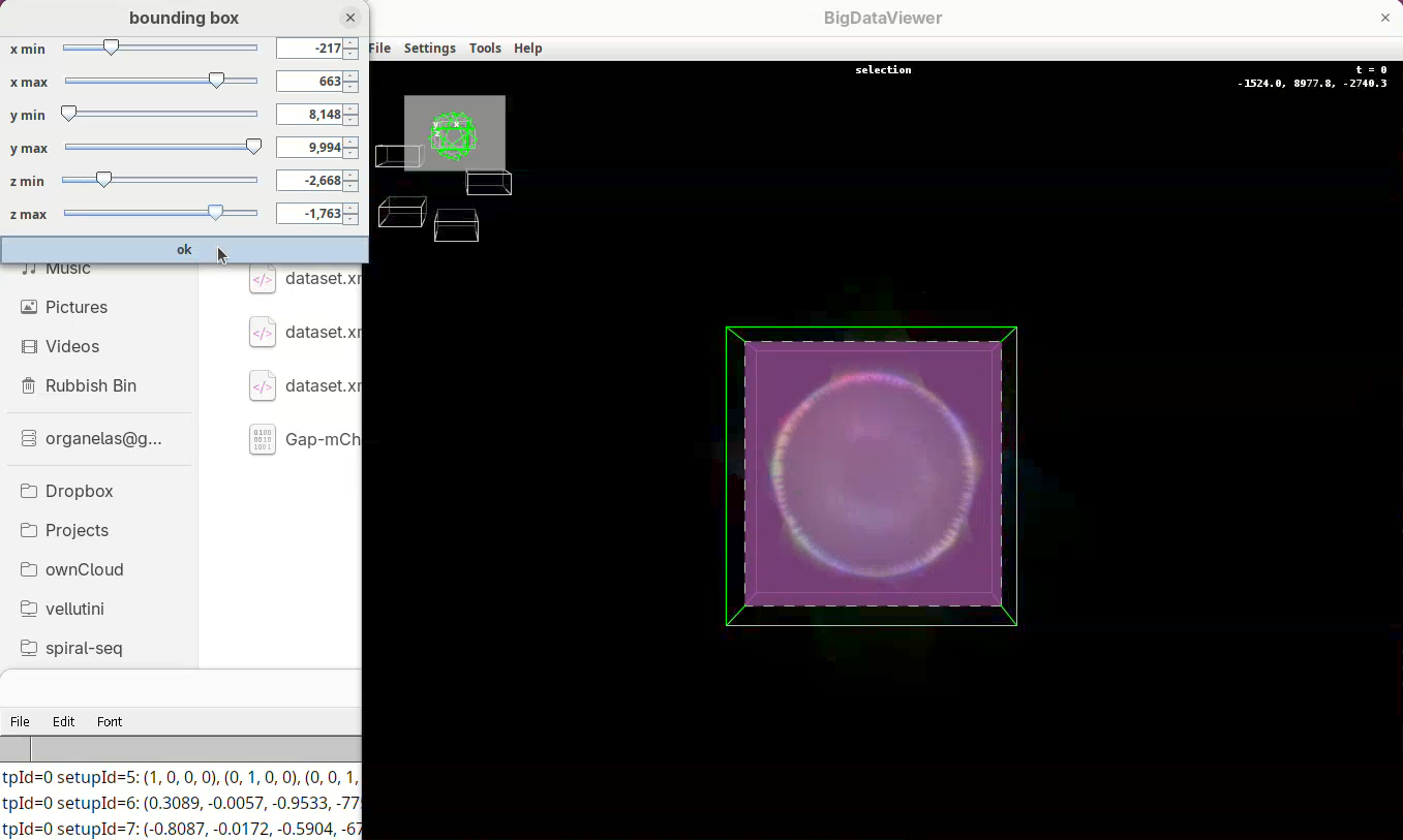
Next we want to cut a bit from the top and bottom regions.

• Move the slider y min to cut from the top and y max to cut from the bottom.

Remember to go through Z to make sure it is not cutting the tip off the embryo (it happens).

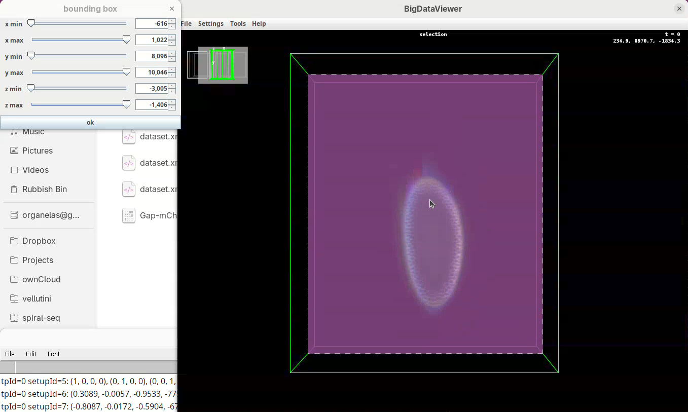
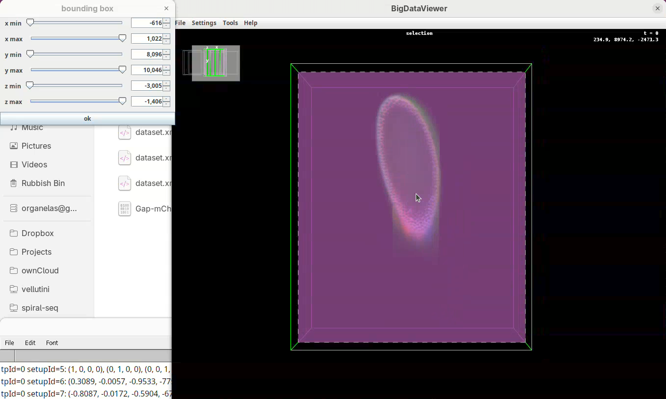
• Finally, press Shift+Y to cut out the exceeding portions in the Z direction.

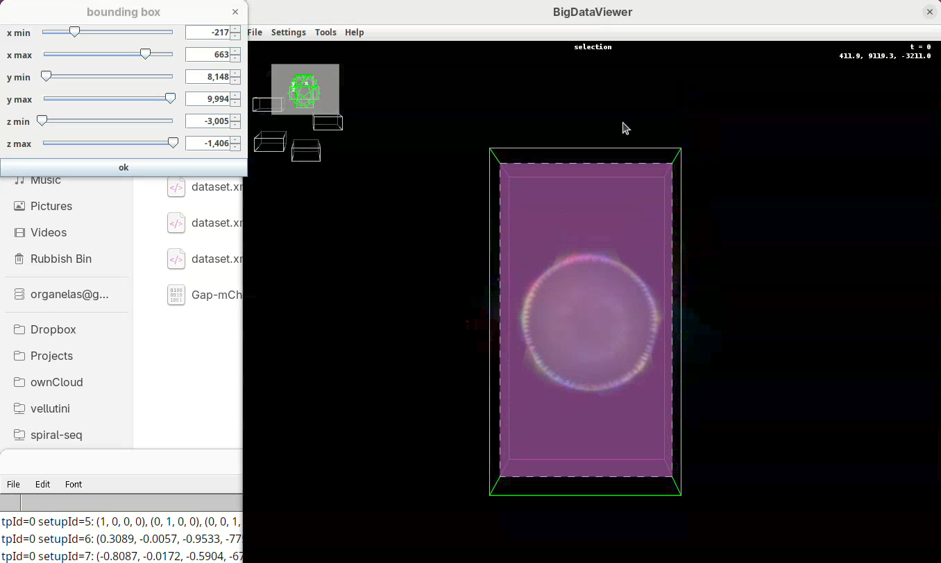
• Use z min to cut from the top (in this orientation) always going through Y to check!
• Then adjust z max to cut from the bottom (in this orientation), also going through Y.

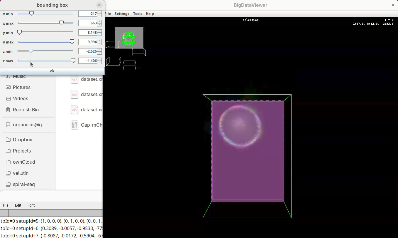
• When done, press OK in the bounding box window.

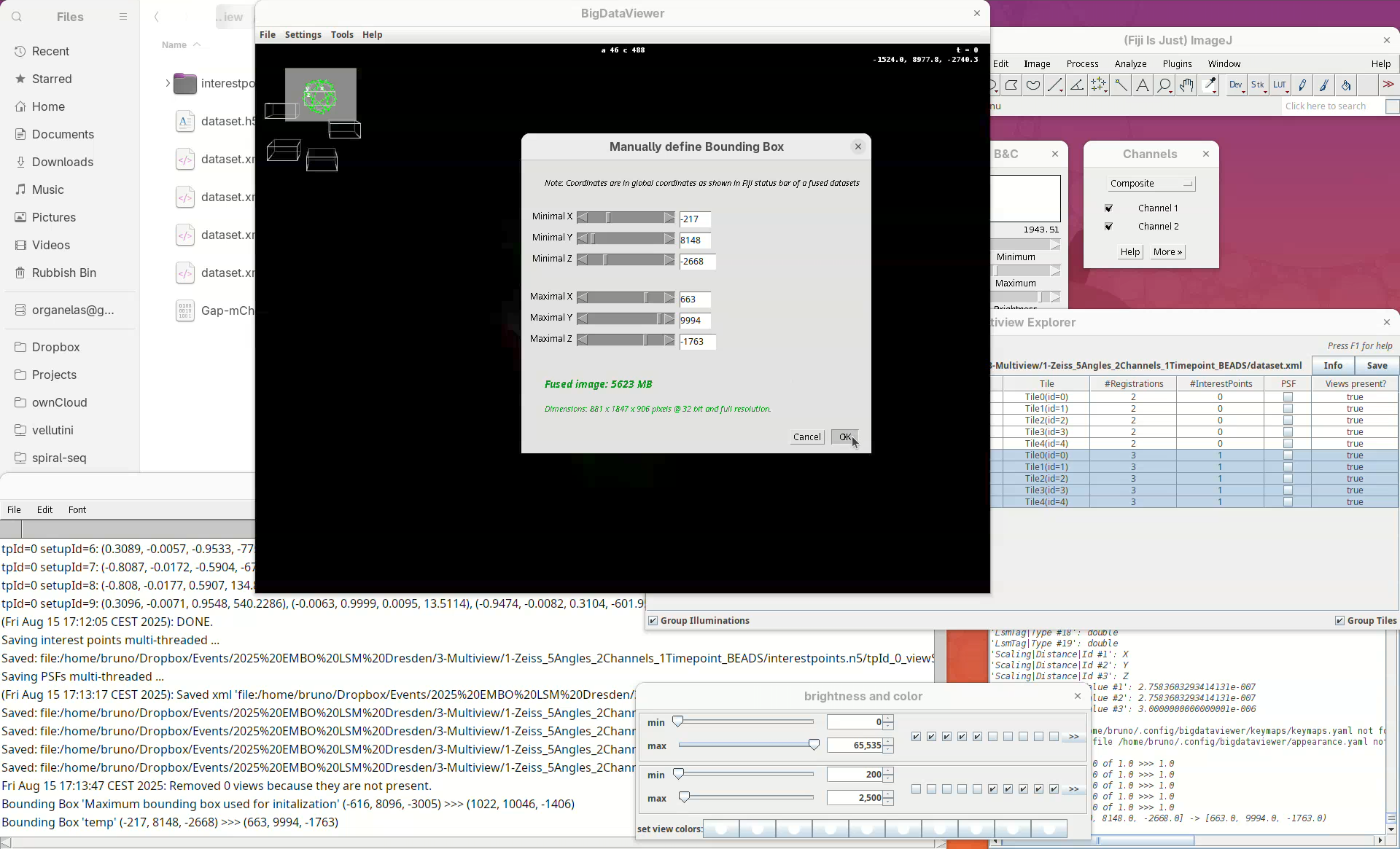
The dimensions of the interactively defined bounding box and the estimated size of the fused image will appear.

• Press OK and Save.

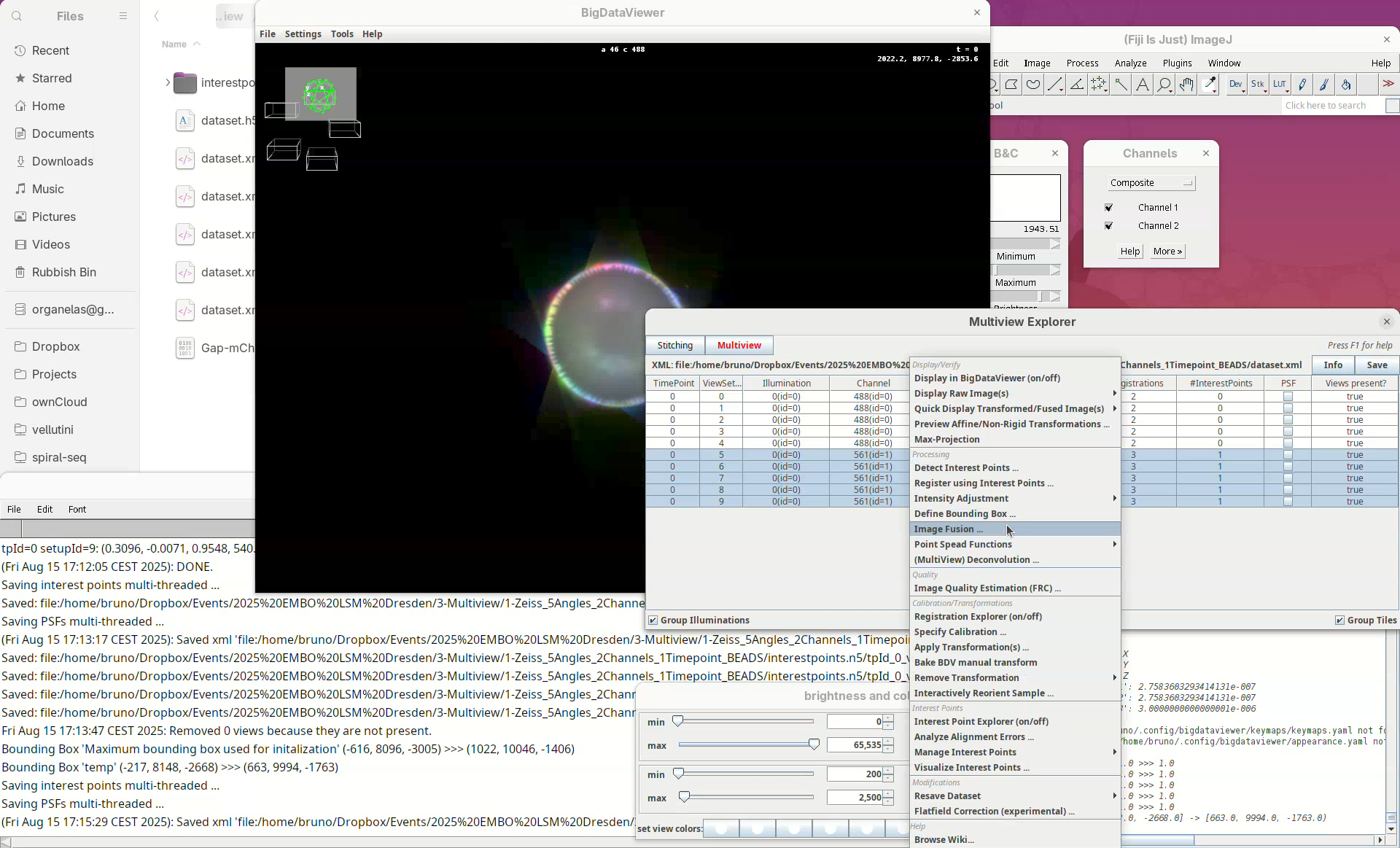
Fuse dataset (one channel)

Finally, let’s begin the fusing of registered views.

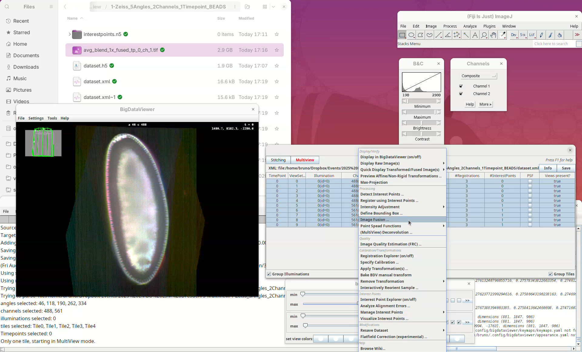
• Select the five registered views in the Multiview Explorer, right-click and press Image Fusion....

The window with fusion options will appear.

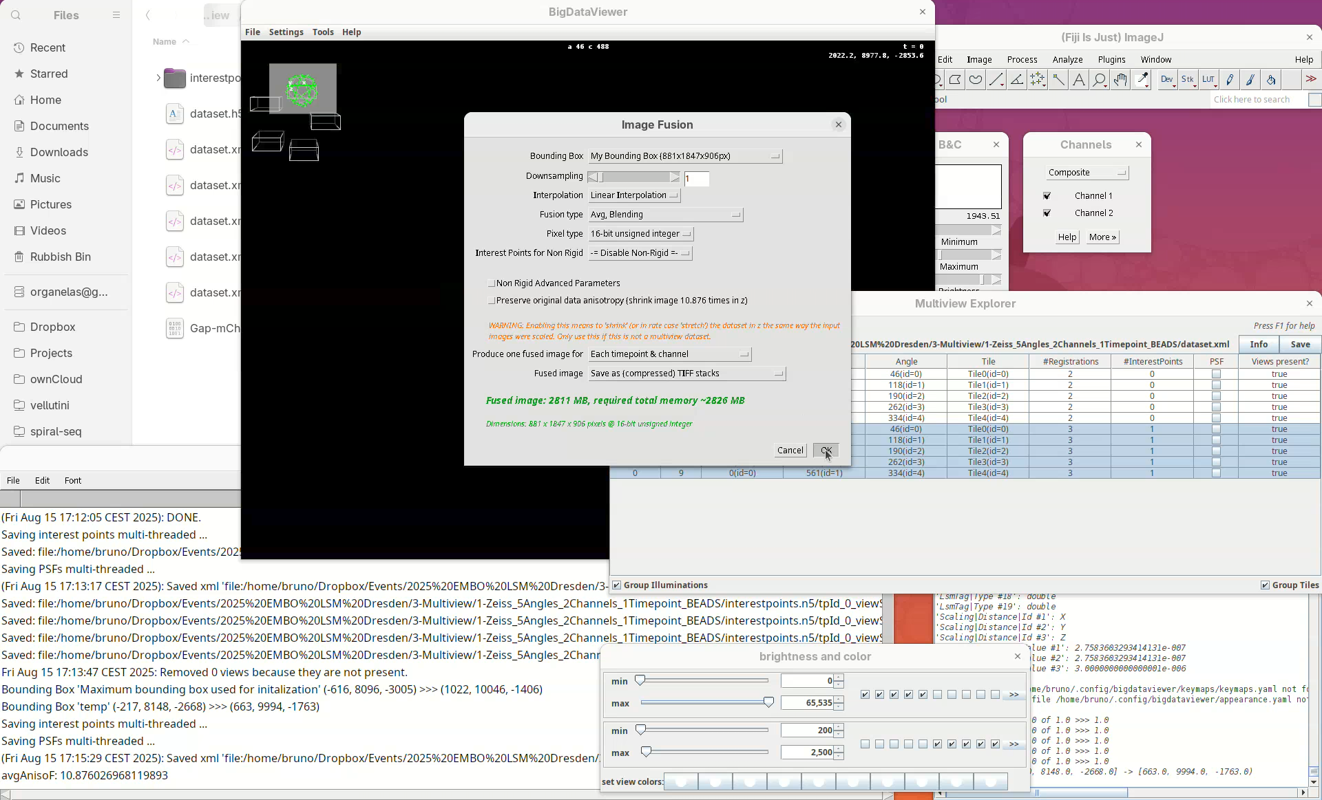
Our “My Bounding Box” is automatically selected for the Bounding Box.

We can choose to downsample the fused image. I highly recommend downsampling 2x, 4x, or even 8x, when fusing a dataset for the first time. Fusing without downsampling (1x) can take a really long time for large samples (many hours), so it is good practice to downsample the fused image to make sure the fusing parameters are good for the dataset before fusing the whole thing.

• For this tutorial, leave Downsampling at 1x.
• For Interpolation keep Linear interpolation, as it gives better outputs.

The Fusion type is an important parameter to choose wisely.

1. The simplest is Avg, which averages the signal of every view per pixel. This is quick but it is combining the good contrast of one view with the blurred side of another view and the resulting contrast will be suboptimal.
2. Avg, Blending is the same as Avg, but it blends smoothly the edges of the different views giving a slightly better fusing than simple Avg.
3. Avg, Blending & Content Based improves the other two options by adding a step that checks and keeps only the best information for each coordinate (keep good contrast, discard blurred information). This option gives the best results. However, it is also the one that requires more memory and takes longer to finish (much longer).

A sane start would be 2x or 4x downsample using Avg, Blending before trying less downsampling and the content based fusion.

• For this tutorial, set Fusion type to Avg, Blending.

For the Pixel type I often use 16-bit, but it depends on what the goal of the fused image is. If it is only to have a volume visualization, 8-bit might be enough. If further processing and analysis is expected, definitely go for 16-bit or, in special cases, 32-bit.

• Set Pixel type to 16-bit unsigned integer.

BigStitcher also has an option for using the interest points information during the fusion step to obtain better results (Interest Points for Non-Rigid). This is a newer feature for advanced use cases and I have not tried it enough to have an opinion about it.

• Leave Interest Points for Non-Rigid as -= Disable Non-Rigid =-.

Generally, we want to have one fused image per timepoint per channel.

• Set Produce one fused image for to Each timepoint & channel.

And I always save the fused image to TIFF stacks. Choosing Display using ImageJ can be dangerous as the fused image will be large and the computer can run out of memory and crash. Writing to disk is safer.

• Set Fused image to Save as (compressed) TIFF stacks.

• Press OK.

• A window with min/max levels will open.

• Press OK.

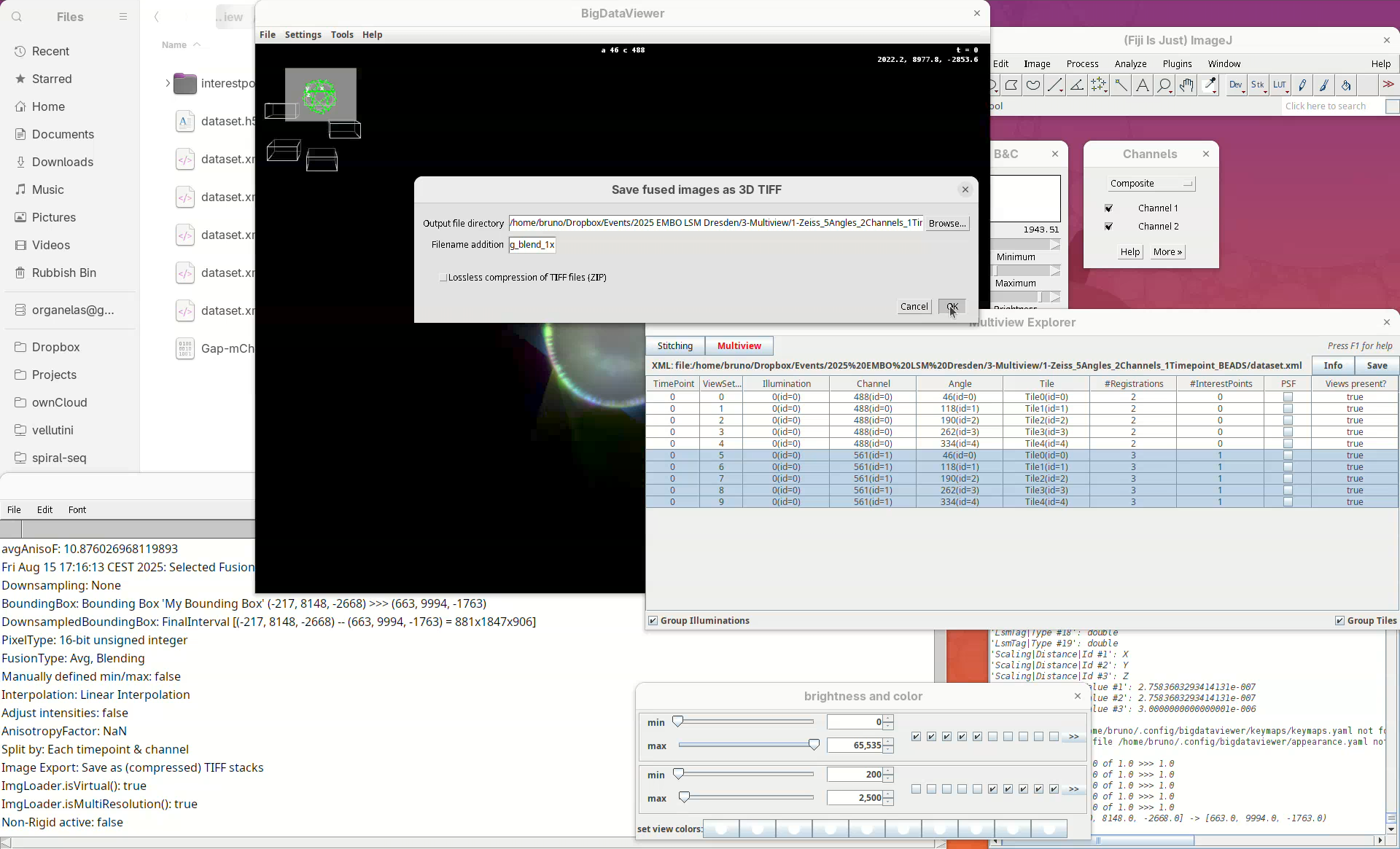
The output directory is the same where the dataset.xml is. We can add a prefix to the filename to distinguish different types of fusion and downsampling (useful when doing it multiple times).

• Set Filename addition to avg_blend_1x.
• Press OK and fusion will start.

When done, open the fused dataset in Fiji.

• Drag and drop the file avg_blend_1x_fused_tp_0_ch_1 into Fiji’s window.
• Then, adjust the contrast to see the data.

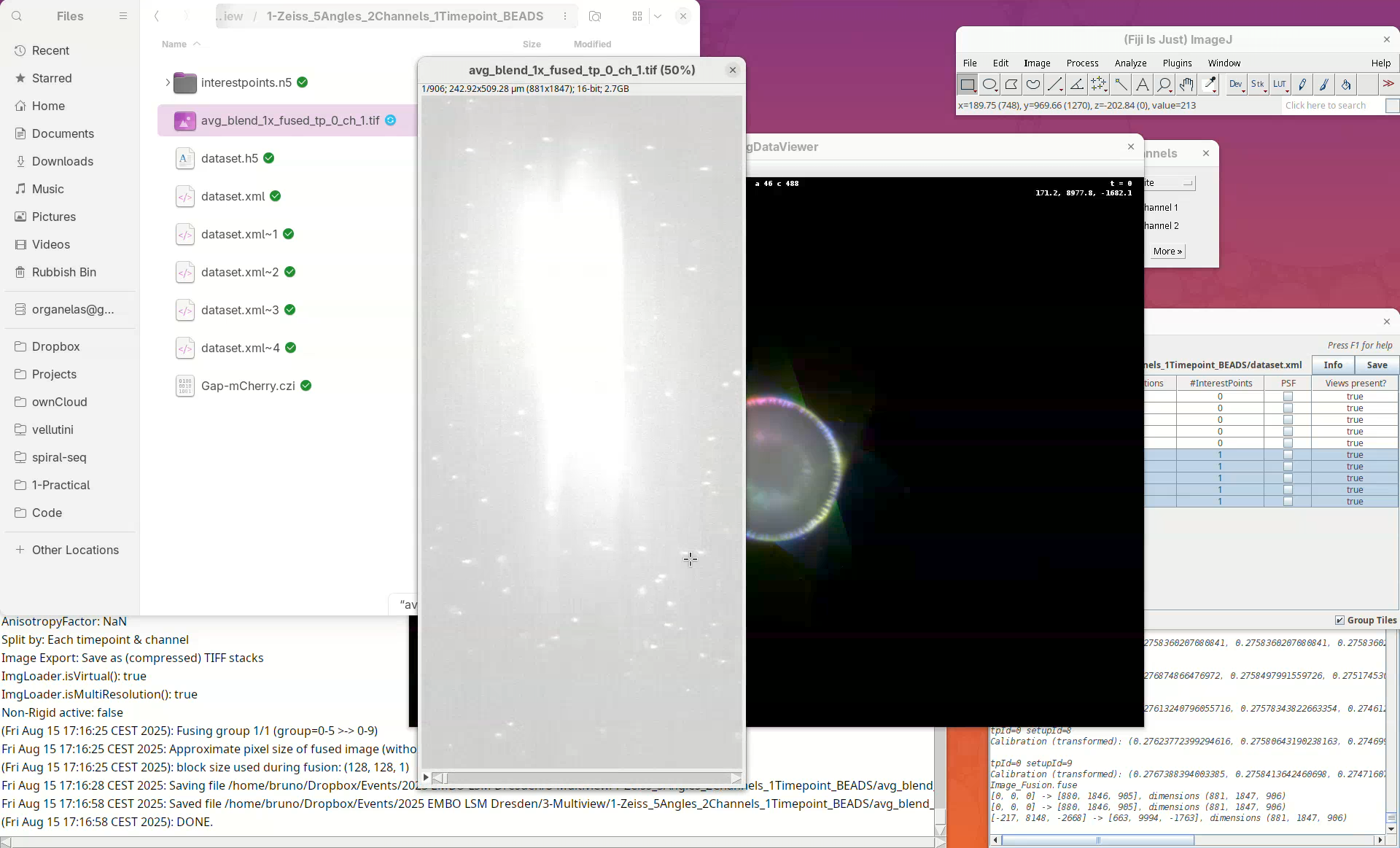
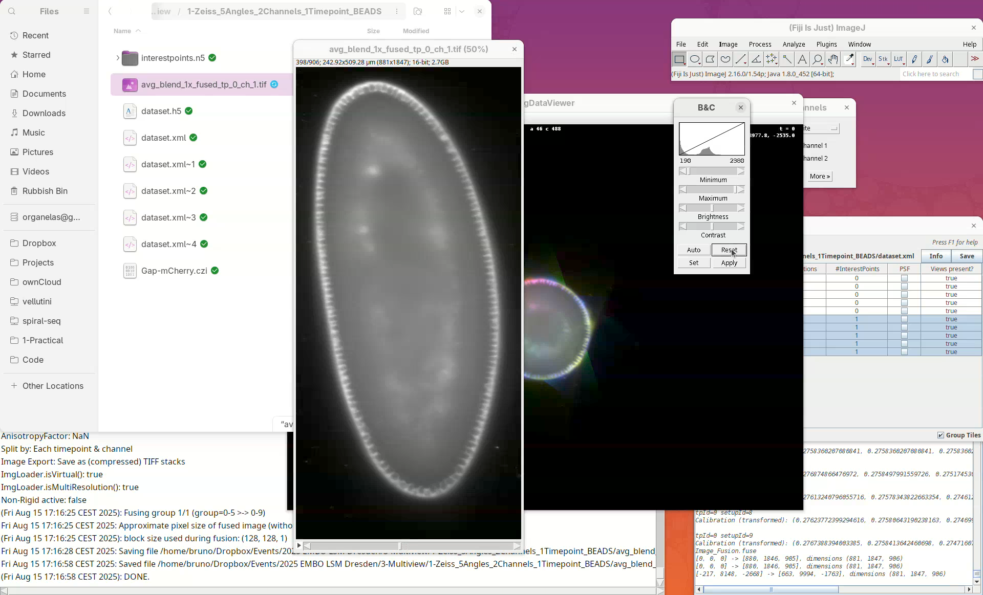
Inspect the fusion result, checking for artifacts. If the sample has a membrane staining, for example, check for doubled membranes.

• Check the fused dataset with the Orthogonal Views.

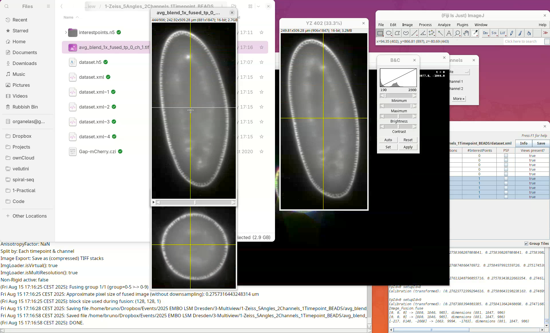
Note that the resulting fused image is isotropic.

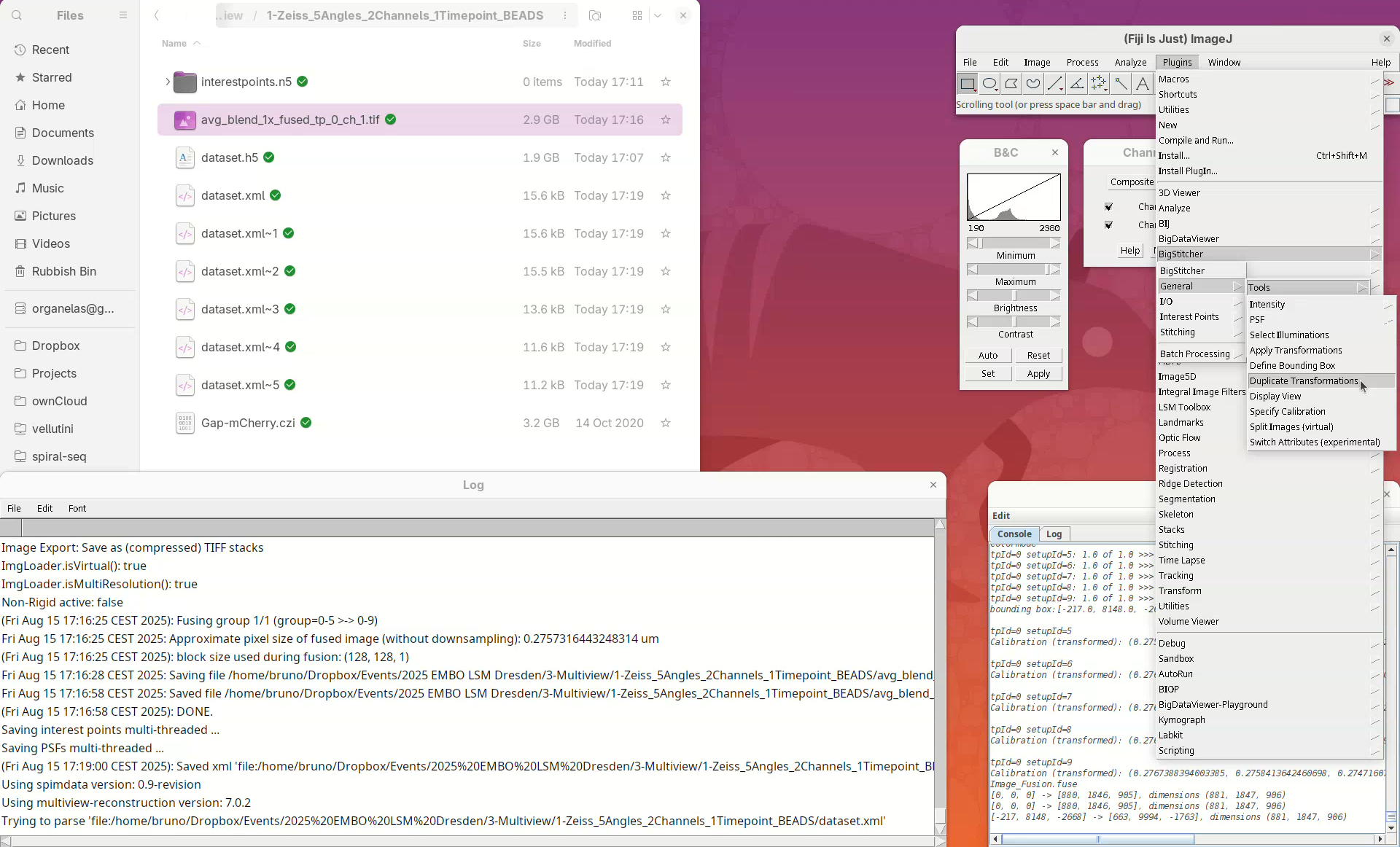
Duplicate transformation

Now that we have successfully registered and fused the views of one channel, we can simply apply the series of transformations to the other channel without the need to detect interest points or register the channel independently.

We can do so using the tool Duplicate Transformations from BigStitcher.

• First, take a note of which channel we have registered (it’s the 561).
• Then, close the Multiview Explorer and the Select dataset window that pops up.
• Finally, go to Plugins > BigStitcher > General > Tools > Duplicate Transformations.

• Select the option One channel to other channels.

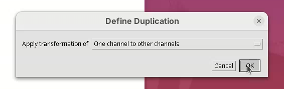
A Select dataset window will open with the last dataset.xml already opened.

• Press OK.

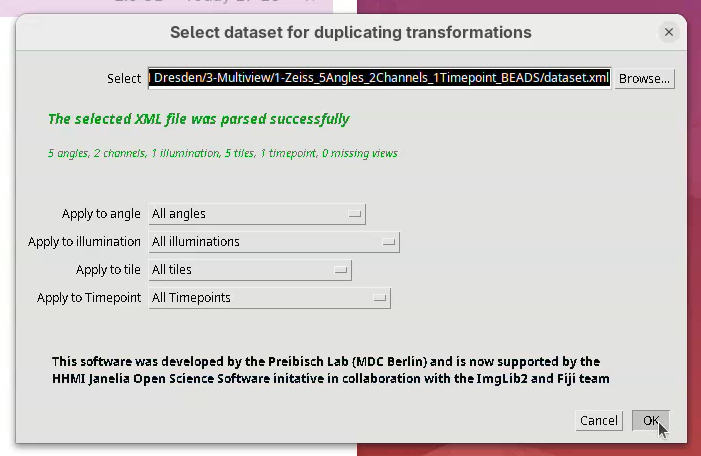
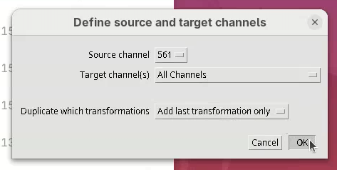
• Set the Source channel to 561.
• Set Target channel(s) to All Channels (all the other channels except for the source one).

The last option, Duplicate which transformations is important. Generally, Replace all transformations works for most cases. However, I often prefer to use Add last transformation only. This will take the last transformation from the source channel and apply it to the target channel. For this to work, however, the source channel can only be one transformation ahead of the target. If, for instance, we had run two subsequent transformations on the source channel, then applied only the last one to the other channels, we would not entirely duplicate all the transformations between the channels. So, always check the #Registrations in the Multiview Explorer to be sure if only the last duplication would work, or simply replace all transformations.

• For now, set Duplicate which transformations to Add last transformation only.
• Press OK.

The transformations will be applied and recorded in the XML file. It’s quick.

• Open BigStitcher again and check if the 5 views of the other channel are registered (they should be).

Fuse dataset (all channels)

We now have both channels registered, but only one was fused.

• To fuse both channels select all the views in the Multiview Explorer, right-click, and select Image Fusion....

• Set the desired parameters for fusion (optimized previously) and run the fusion again as described above.

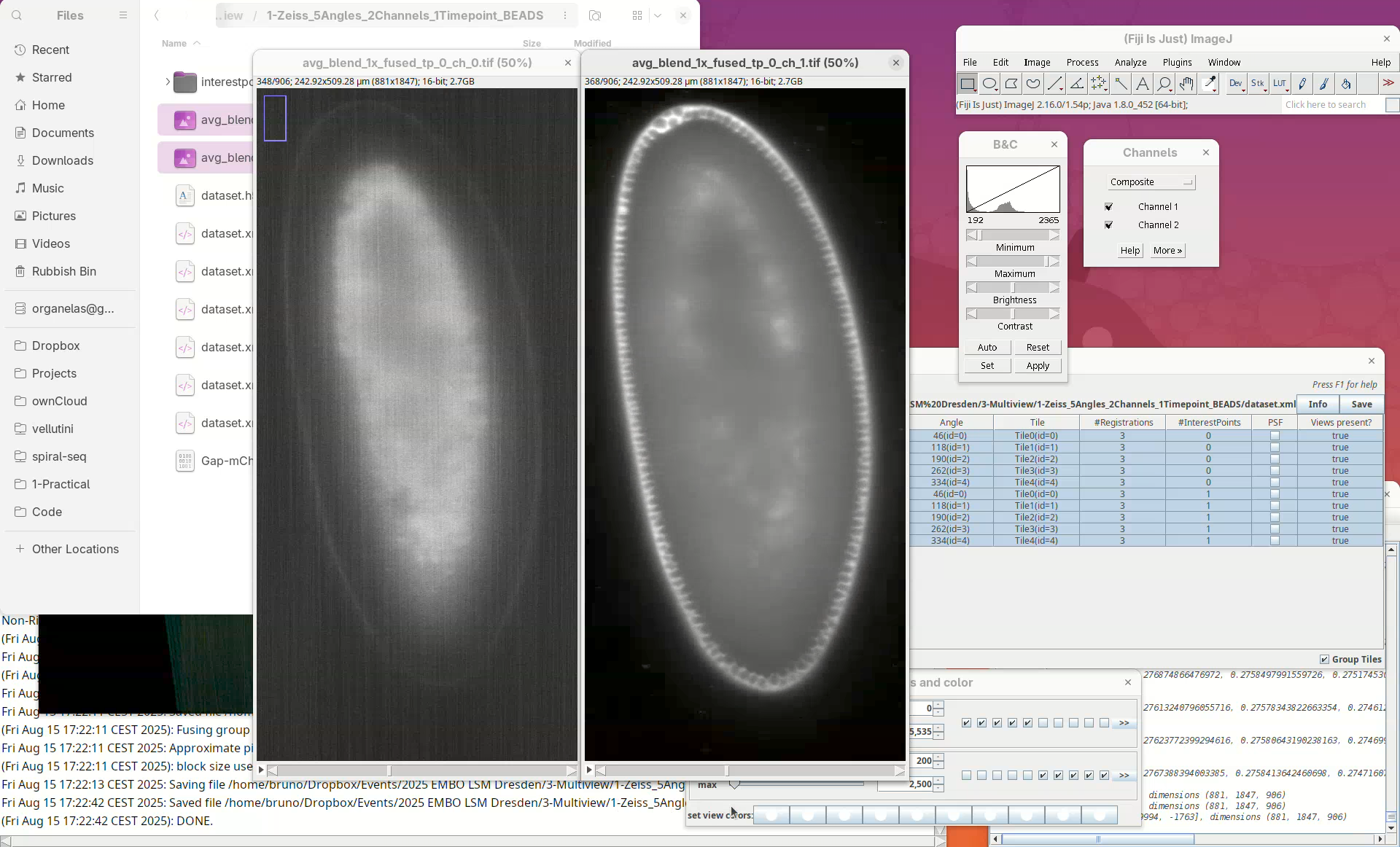
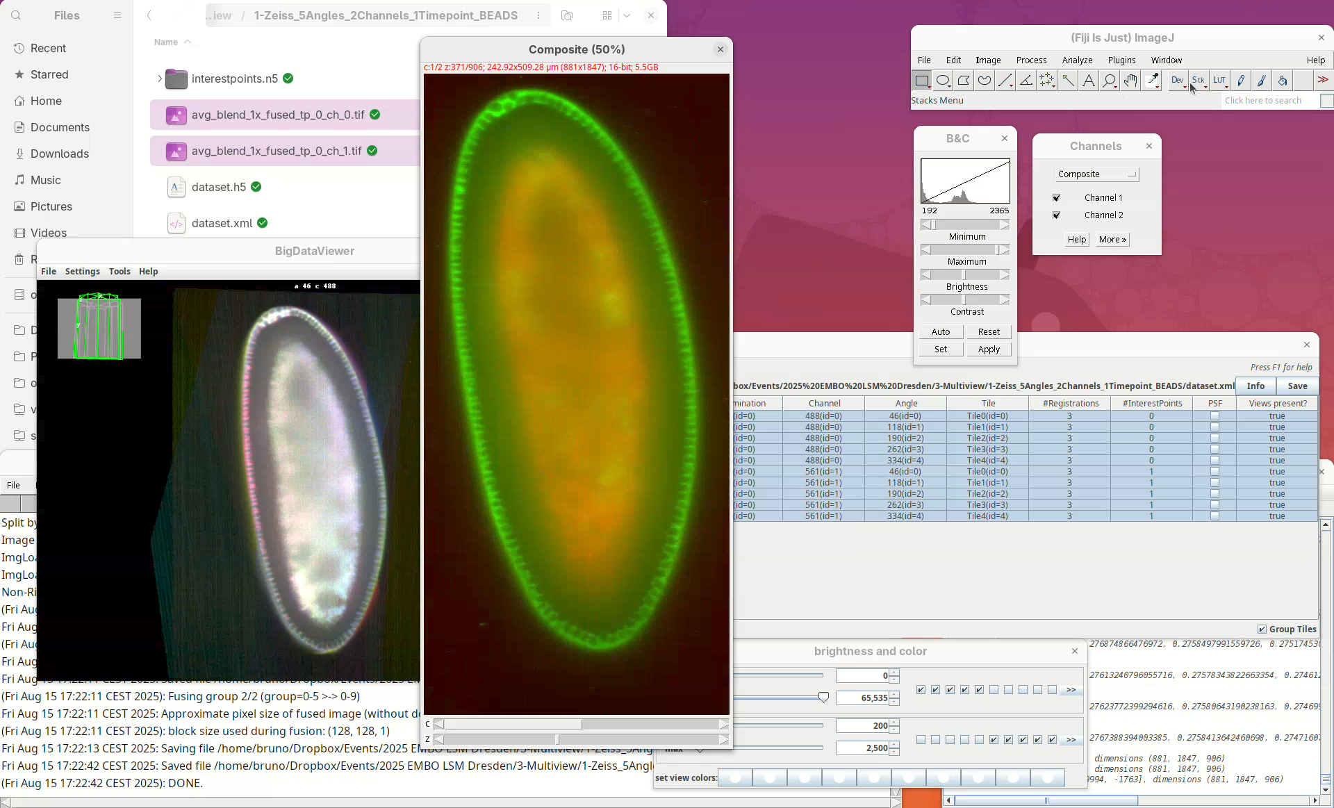
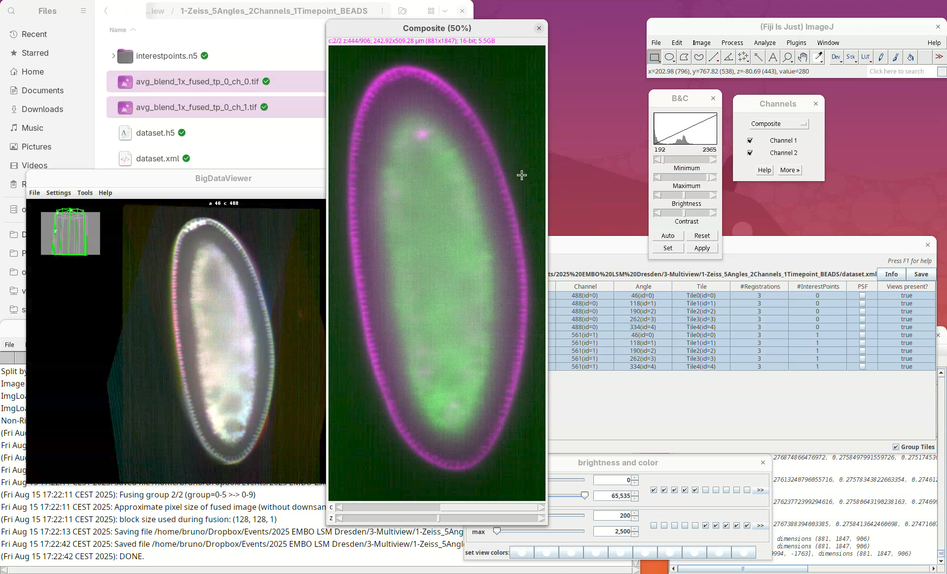
This time there will be two files as output: avg_blend_1x_fused_tp_0_ch_0.tif and avg_blend_1x_fused_tp_0_ch_1.tif.

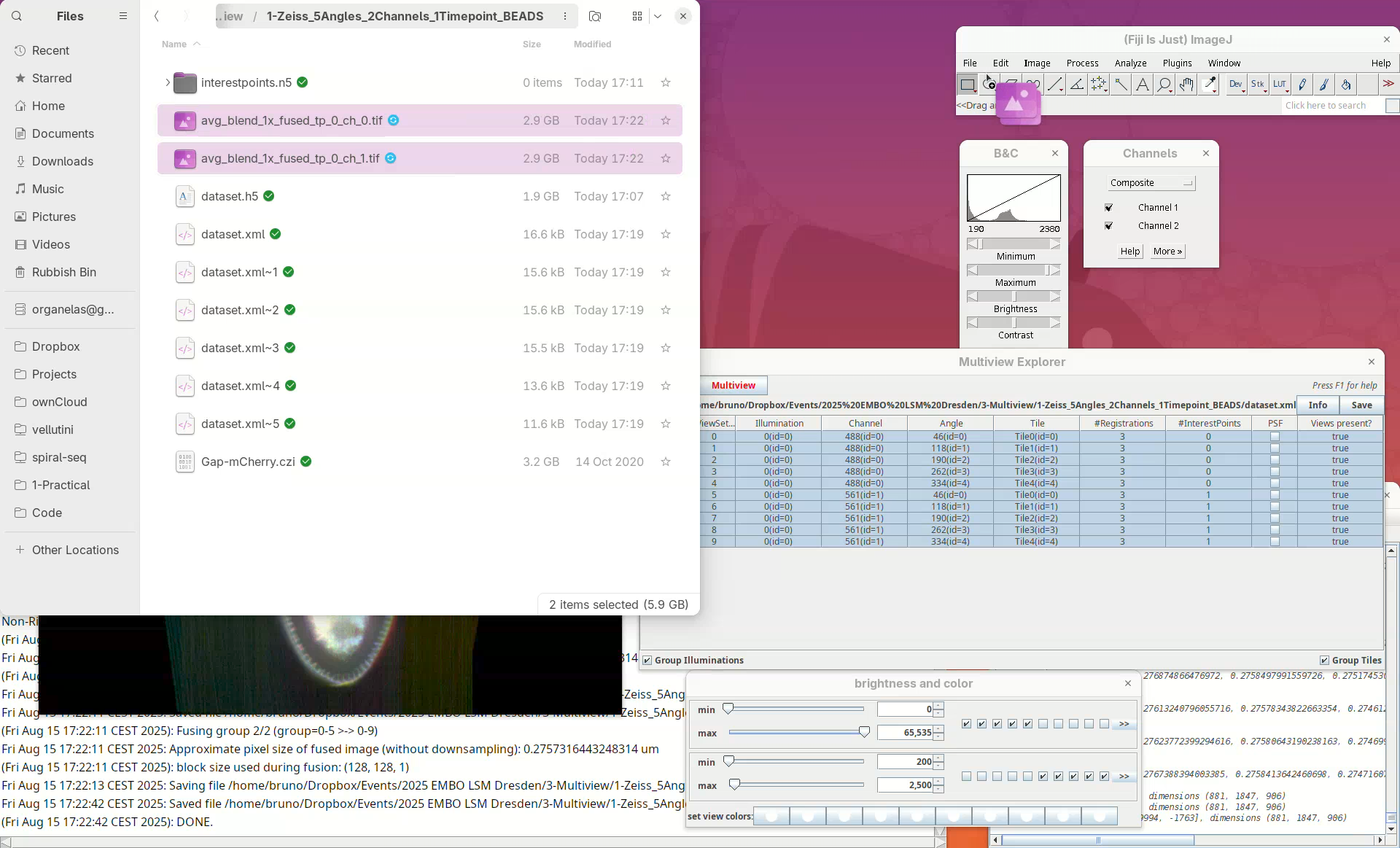
• Open both files in Fiji and adjust their contrast.

• Then go to Image > Color > Merge Channels....

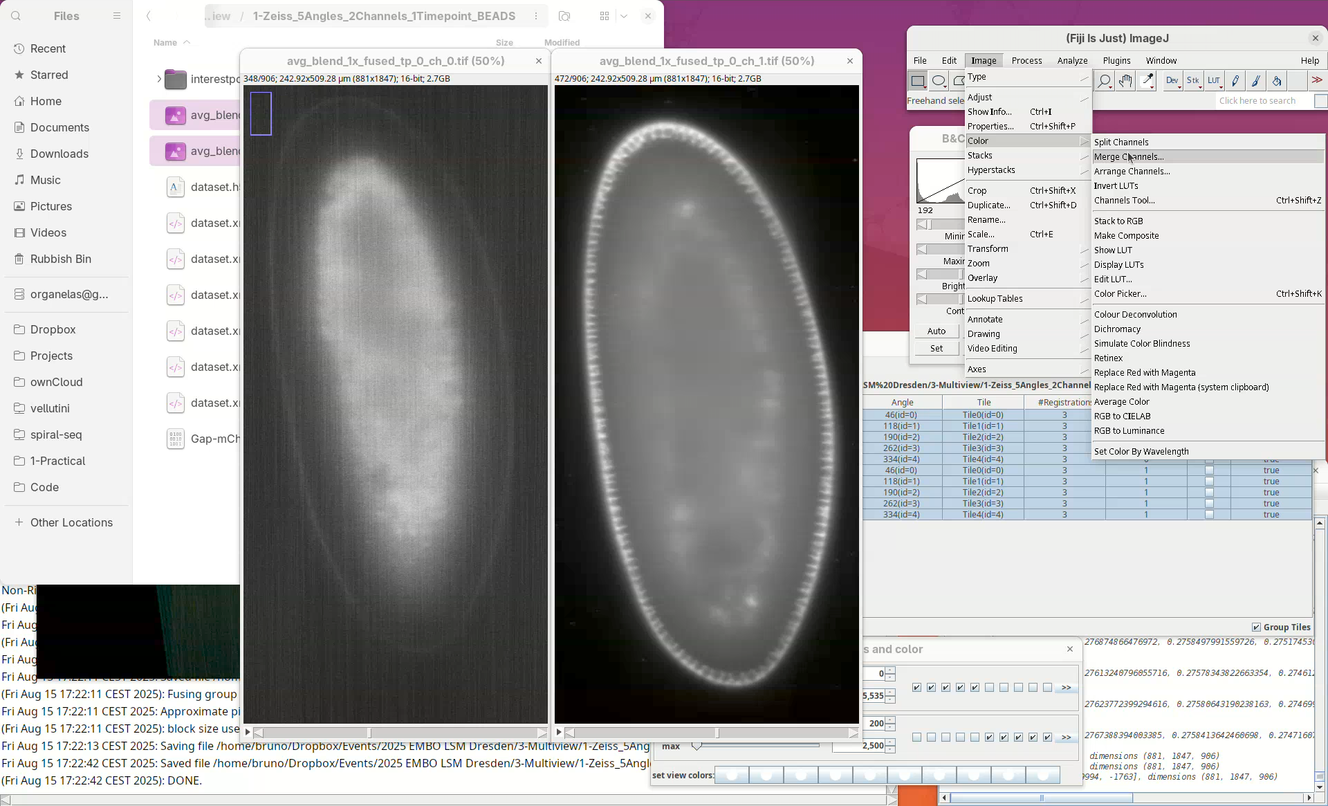
• Select ch_0 for C1 and ch_1 for C2 and press OK.

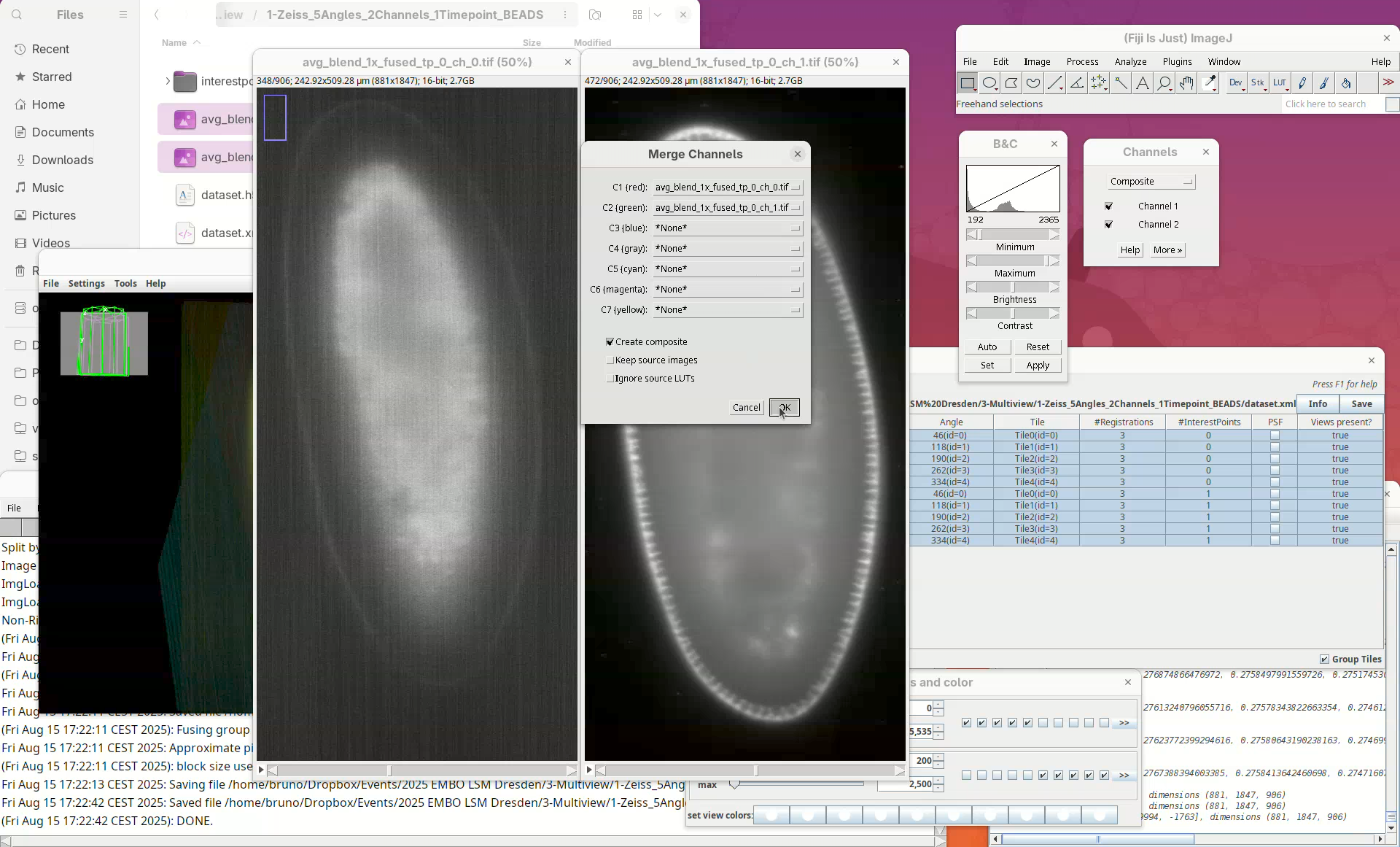
A red-green 2-channel stack will open. But, red-green combination isn’t good.

• Update the red to magenta using the LUT tool.

We can even compare this fused dataset with one of the views of the original dataset.

• Drag and drop the CZI file, select the first view only to import, and put the stacks side-by-side for a comparison slice by slice.

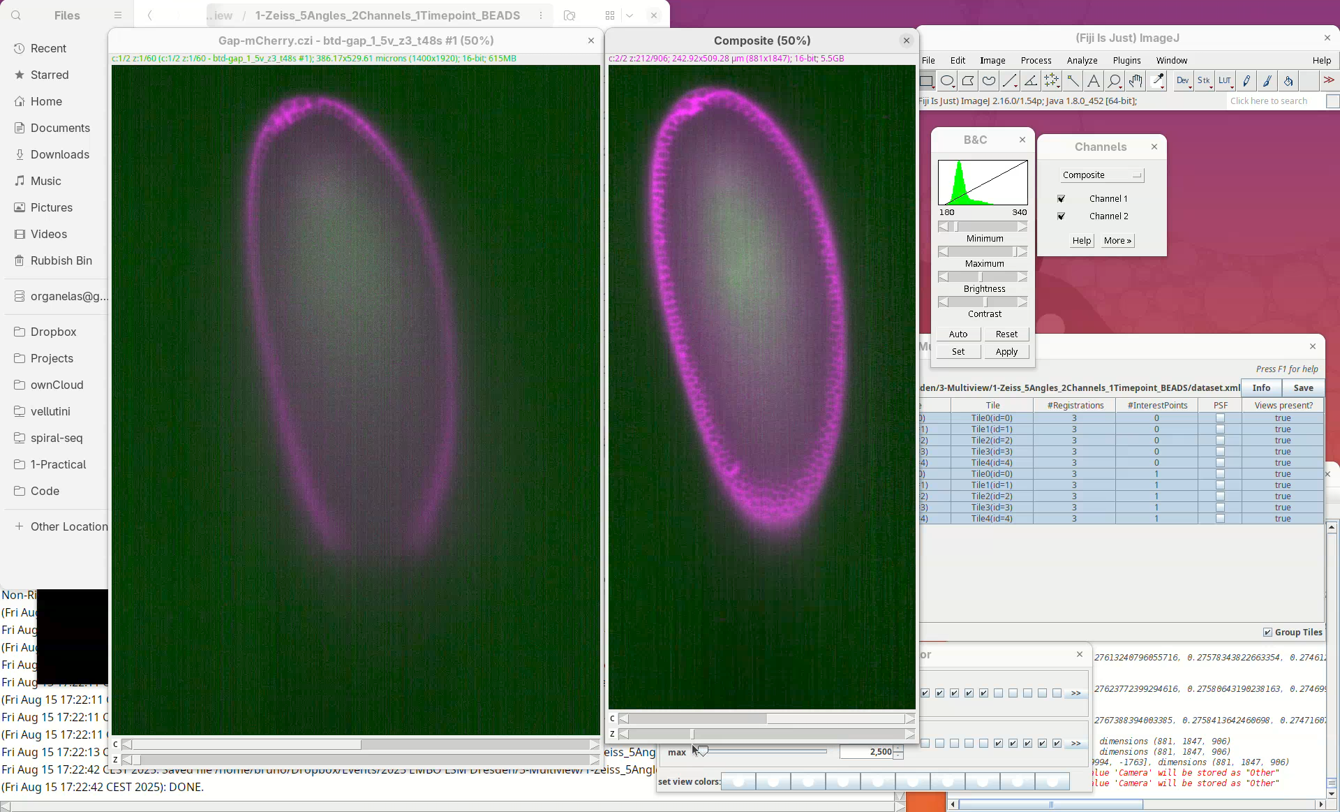
Note how the missing data in the single view is nicely present in the fused dataset.

Citation

Vellutini, B. C. (2026). Multiview reconstruction in Fiji using BigStitcher. Zenodo. https://doi.org/10.5281/zenodo.18090752

License

This tutorial is available under a Creative Commons Attribution 4.0 International License.

References

Hörl, David, Fabio Rojas Rusak, Friedrich Preusser, Paul Tillberg, Nadine Randel, Raghav K Chhetri, Albert Cardona, et al. 2019. “BigStitcher: Reconstructing High-Resolution Image Datasets of Cleared and Expanded Samples.” Nat. Methods 16 (September): 870–74. https://doi.org/10.1038/s41592-019-0501-0.

Pietzsch, Tobias, Stephan Saalfeld, Stephan Preibisch, and Pavel Tomancak. 2015. “BigDataViewer: Visualization and Processing for Large Image Data Sets.” Nat. Methods 12 (June): 481–83. https://doi.org/10.1038/nmeth.3392.

Preibisch, Stephan, Stephan Saalfeld, Johannes Schindelin, and Pavel Tomancak. 2010. “Software for Bead-Based Registration of Selective Plane Illumination Microscopy Data.” Nat. Methods 7 (June): 418–19. https://doi.org/10.1038/nmeth0610-418.

Schindelin, Johannes, Ignacio Arganda-Carreras, Erwin Frise, Verena Kaynig, Mark Longair, Tobias Pietzsch, Stephan Preibisch, et al. 2012. “Fiji: An Open-Source Platform for Biological-Image Analysis.” Nat. Methods 9 (June): 676–82. https://doi.org/10.1038/nmeth.2019.

Vellutini, Bruno C. 2025. “Fly Embryo Multiview Lightsheet Dataset.” Zenodo. https://doi.org/10.5281/zenodo.18078061.